查看神经网络

import keras_metrics as km
from keras.engine.saving import load_model
dependencies = {
        'categorical_precision': km.categorical_precision(),
        'categorical_recall':km.categorical_recall(),
        'categorical_f1_score':km.categorical_f1_score()
}
model = load_model("D:/Users/JiajunBernoulli/MyProject/Tigers/stripes_detection_by_keras/right/models/ResNet34_0_1/tiger.models.h5", custom_objects=dependencies)

model.summary()

需要注意input_1为第0层，而不是第1层。

获得目标层

通过查看神经网络，可以找到目标层的索引，再通过索引来获取目标层。

import keras_metrics as km
from keras.engine.saving import load_model
dependencies = {
        'categorical_precision': km.categorical_precision(),
        'categorical_recall':km.categorical_recall(),
        'categorical_f1_score':km.categorical_f1_score()
}

model = load_model("D:/Users/JiajunBernoulli/MyProject/Tigers/stripes_detection_by_keras/right/models/ResNet34_0_2/tiger.models.h5", custom_objects=dependencies)
# redefine model to output right after the first hidden layer
ixs=[2, 4]
outputs = [model.layers[i].output for i in ixs]
for output in outputs:
        print(output)

获得了第二层和第四层。

卷积与池化对比

加载图片

# load the image with the required shape
img = load_img('./images/bird.jpg', target_size=(224, 224))
img = img_to_array(img)
img = expand_dims(img, axis=0)
img = preprocess_input(img)

预测图片

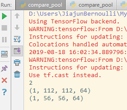
根据加载的模型和图片进行预测，得到的是一个四维数组，第一维对应不同的隐藏层，二三维对应图片像素，第四维对应同一层不同filter的结果。

# get feature map for first hidden layer
model = Model(inputs=model.inputs, outputs=outputs)
feature_maps = model.predict(img)
print(len(feature_maps))

conv_map=feature_maps[0]
print(conv_map.shape)‘

pool_map=feature_maps[1]
print(pool_map.shape)

目标层只有两个，预测的输出也只有两个。

保存结果

直接保存可以保持原尺寸，以便看出池化后的大小变化，绘图的话需要调整像素才能保持原尺寸很麻烦。

pyplot.imsave("conv_map.png",conv_map[0, :, :, 0], cmap='gray')
pyplot.imsave("pool_map.png",pool_map[0, :, :, 0], cmap='gray')

很容易看出池化的效果

不同filter的对比

这个代码源自国外的一个网友，我简单修改了一下。

# visualize feature maps output from each block in the vgg model
from keras.applications.vgg16 import VGG16
from keras.applications.vgg16 import preprocess_input
from keras.engine.saving import load_model
from keras.preprocessing.image import load_img
from keras.preprocessing.image import img_to_array
from keras.models import Model
from matplotlib import pyplot
from numpy import expand_dims
import keras_metrics as km
# load the model
dependencies = {
        'categorical_precision': km.categorical_precision(),
        'categorical_recall':km.categorical_recall(),
        'categorical_f1_score':km.categorical_f1_score()
}

model = load_model("D:/Users/JiajunBernoulli/MyProject/Tigers/stripes_detection_by_keras/right/models/ResNet34_0_2/tiger.models.h5", custom_objects=dependencies)
# redefine model to output right after the first hidden layer
ixs = [2, 5, 7]
outputs = [model.layers[i].output for i in ixs]
# load the image with the required shape
img = load_img('./images/bird.jpg', target_size=(224, 224))
img = img_to_array(img)
img = expand_dims(img, axis=0)
img = preprocess_input(img)

# get feature map for first hidden layer
model = Model(inputs=model.inputs, outputs=outputs)
feature_maps = model.predict(img)

# plot the output from each block
square = 8
for fmap in feature_maps:
	# plot all 64 maps in an 8x8 squares
	ix = 1
	for _ in range(square):
		for _ in range(square):
			# specify subplot and turn of axis
			ax = pyplot.subplot(square, square, ix)
			ax.set_xticks([])
			ax.set_yticks([])
			# plot filter channel in grayscale
			# print(fmap.shape)
			pyplot.imshow(fmap[0, :, :, ix-1], cmap='gray')
			ix += 1
	# show the figure
	pyplot.show()