在上篇的tf.keras快速入门——函数式API中简单的使用了和序列模型不同的样子来定义网络。但是,该网络只是层与层之间的连接更加灵活,但却没有其余的优点了。当我们需要完全自定义网络模型和前向传递过程,就满足不了了。
这里,我们讨论自定义模型。
自定义Model类,需要最少复写两个方法,分别是:
__init__()call()
在__init__()我们初始化所需要的神经网络层,在call()中定义这些神经网络层如何连接,可以理解为前向传播。然后需要返回一个outputs,也就是输出。
在本篇中,还是考虑修改鸢尾花分类案例。
在上篇中,我们是这样定义的:
input_data = tf.keras.Input(shape=(len(x_data[0],)))
h_1 = tf.keras.layers.Dense(4, activation="relu")(input_data)
h_2 = tf.keras.layers.Dense(3, activation="softmax")(h_1)
在这里还是保留类似的结构:
import matplotlib.pyplot as plt
%matplotlib inline
import tensorflow as tf
from sklearn.datasets import load_iris
# 训练集和测试集的划分
from sklearn.model_selection import train_test_split
x_data = load_iris().data # 特征,【花萼长度,花萼宽度,花瓣长度,花瓣宽度】
y_data = load_iris().target # 分类
x_train, x_test, y_train, y_test = train_test_split(x_data, y_data, test_size=0.30, random_state=42)
class MyModel(tf.keras.Model):
def __init__(self, hidden_shape, output_shape):
super(MyModel, self).__init__()
self.layer1 = tf.keras.layers.Dense(hidden_shape, activation='relu')
self.layer2 = tf.keras.layers.Dense(output_shape, activation='softmax')
def call(self, inputs):
h1 = self.layer1(inputs)
out = self.layer2(h1)
return out
model = MyModel(hidden_shape=4, output_shape=3)
model.compile(optimizer=tf.keras.optimizers.Adam(),
loss=tf.keras.losses.sparse_categorical_crossentropy,
metrics=['accuracy'])
history = model.fit(x_train, y_train, epochs=300)
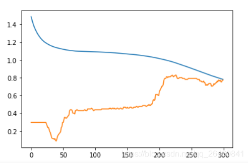
for key in history.history.keys():
plt.plot(history.epoch, history.history[key])