傅里叶变换的应用涵盖了概率与统计、信号处理、量子力学和图像处理等学科。
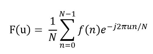
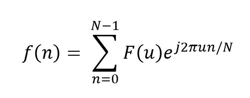
离散傅里叶变换的公式如下:
在MATLAB中,可以直接使用函数库fft(X)对一维向量X做傅里叶变换,分析信号的组成。如下例子处理一维离散信号
信号分析
通过傅里叶变换,可以将实变信号f(t)分解成各个频率分量的线性叠加,进而从频率的角度研究信号的组成。
来看这个杂乱无章的曲线图,你是否能看出它的规律?
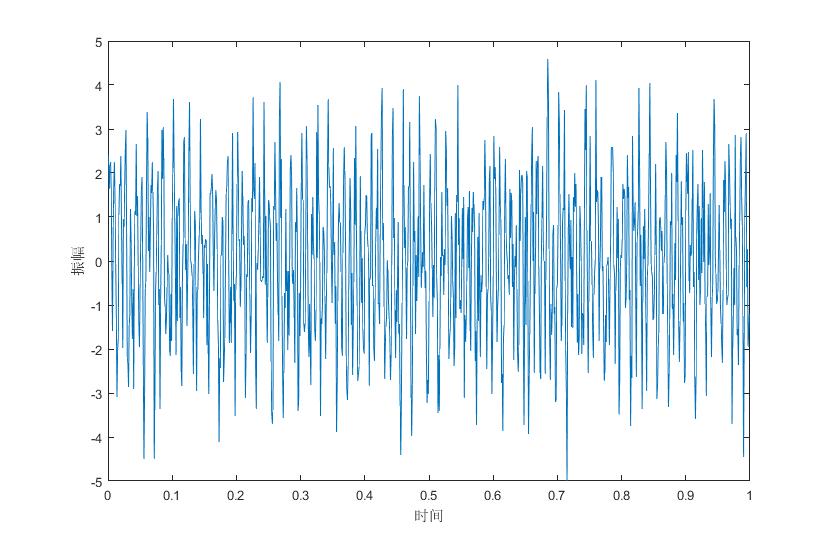
Figure 1 What's the law of the signal?
让我们来对它做一维离散傅里叶变换,得到下图:
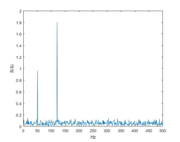
Figure 2 The Fourier Transform of the signal in the figure 1
从图2的傅里叶变换中我们可以观察到信号在频率为50Hz和120Hz的地方有峰值,表明了原信号主要由频率为50Hz和120Hz的三角函数信号组成。
上面例子的具体MATLAB代码如下:
clear
Fs = 1000;            % Sampling frequency
T = 1/Fs;             % Sampling period
L = 1000;             % Length of signal
t = (0:L-1)*T;        % Time vector

S = 0.9*sin(2*pi*50*t) + 1.8*sin(2*pi*120*t); %standard signal
X = S + 1*randn(size(t)); %there are some noise mixing in the signal.

Y = fft(X);           % Fourier Transform of the signal

f = 1:L/2;            % the frequence of label
                      % half of Y is enough to show the information.
Y = Y./L*2;           % calculate the amplitude of Fourier Transform of the signal

%draw the curve
figure(1);
plot(t,X);            % show the original signal
xlabel('时间')
ylabel('振幅')
figure(2);
plot(f,abs(Y(1:L/2)));% show the Fourier Transform of the signal
xlabel('Hz');
ylabel('振幅');
傅里叶变换可以把信号的振动频率分离出来,我们可以通过设置不同频率分量前的系数,可实现信号的滤波。
如含有噪声的信号:
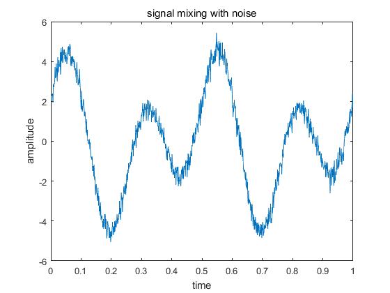
Figure 3 signal mixing with noise
将该信号进行傅里叶变换,然后使得高频信号的系数为零,再傅里叶反变换回原信号,可得到滤波后的结果:
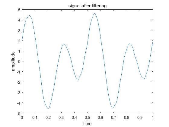
Figure 4 signal after filtering
要注意的是,要想使用好傅里叶变换,必须对傅里叶变换有较为深入的了解,比如上面的滤波中,如果设置滤波频率的界限不同,那么其滤波效果也不同;还要注意的是,傅里叶变换后的信号具有周期性,其数据关于中心位置对称,所以滤波界限要关于中心对称;上例中具体实现代码如下:
clear
Fs = 1000;
T = 1./Fs;
L = 1000;
t = (0:L-1)*T;
S = 2*cos(2*pi*2*t)+3*sin(2*pi*4*t);    %standard signal without the noise
X = S+0.3*randn(size(t));               %signal mixing with noise
figure(1);
plot(t,X);
title('signal mixing with noise');
xlabel('time');
ylabel('amplitude');

Y1 = fft(X);                            %fourier transform

threadhold = 30;                        %setting the filtering threadhold
Y1(threadhold:(L-threadhold)) = 0;      %filtering

X1 = ifft(Y1);                          %Inverse Fourier transform
figure(2);
plot(t,X1);
title('signal after filtering');
xlabel('time');
ylabel('amplitude');
本主要讲了离散傅里叶变换的两个应用——分析信号组成和滤波,其用处还很广泛,比如数据压缩、求微分方程等等。