一、微积分
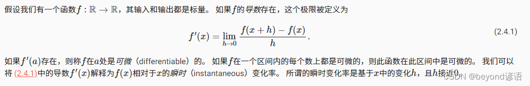
定义函数u = f(x) = 3x² - 4x,求x = 1时的导数
%matplotlib inline
#可以将matplotlib的图表直接嵌入到Notebook之中
import numpy as np
from matplotlib_inline import backend_inline
from d2l import torch as d2l
定义u = f(x) = 3x² - 4x
令x=1,h趋近于0,即u` = 2
def f(x):
    return 3 * x ** 2 - 4 * x
def numerical_lim(f, x, h):
    return (f(x + h) - f(x)) / h
h = 0.1
for i in range(5):
    print(f'h={

      h:.5f}, numerical limit={

      numerical_lim(f, 1, h):.5f}')
    h *= 0.1
"""
h=0.10000, numerical limit=2.30000
h=0.01000, numerical limit=2.03000
h=0.00100, numerical limit=2.00300
h=0.00010, numerical limit=2.00030
h=0.00001, numerical limit=2.00003
"""
use_svg_display()函数指定matplotlib软件包输出svg图表以获得更清晰的图像
#@save是一个特殊的标记,会将对应的函数、类或语句保存在d2l包中
def use_svg_display():  #@save
    """使用svg格式在Jupyter中显示绘图"""
    backend_inline.set_matplotlib_formats('svg')
定义set_figsize函数来设置图表大小
def set_figsize(figsize=(3.5, 2.5)):  #@save
    """设置matplotlib的图表大小"""
    use_svg_display()
    d2l.plt.rcParams['figure.figsize'] = figsize
set_axes函数用于设置由matplotlib生成图表的轴的属性
#@save
def set_axes(axes, xlabel, ylabel, xlim, ylim, xscale, yscale, legend):
    """设置matplotlib的轴"""
    axes.set_xlabel(xlabel)
    axes.set_ylabel(ylabel)
    axes.set_xscale(xscale)
    axes.set_yscale(yscale)
    axes.set_xlim(xlim)
    axes.set_ylim(ylim)
    if legend:
        axes.legend(legend)
    axes.grid()
定义plot函数来简洁地绘制多条曲线
#@save
def plot(X, Y=None, xlabel=None, ylabel=None, legend=None, xlim=None,
         ylim=None, xscale='linear', yscale='linear',
         fmts=('-', 'm--', 'g-.', 'r:'), figsize=(3.5, 2.5), axes=None):
    """绘制数据点"""
    if legend is None:
        legend = []

    set_figsize(figsize)
    axes = axes if axes else d2l.plt.gca()

    # 如果X有一个轴,输出True
    def has_one_axis(X):
        return (hasattr(X, "ndim") and X.ndim == 1 or isinstance(X, list)
                and not hasattr(X[0], "__len__"))

    if has_one_axis(X):
        X = [X]
    if Y is None:
        X, Y = [[]] * len(X), X
    elif has_one_axis(Y):
        Y = [Y]
    if len(X) != len(Y):
        X = X * len(Y)
    axes.cla()
    for x, y, fmt in zip(X, Y, fmts):
        if len(x):
            axes.plot(x, y, fmt)
        else:
            axes.plot(y, fmt)
    set_axes(axes, xlabel, ylabel, xlim, ylim, xscale, yscale, legend)
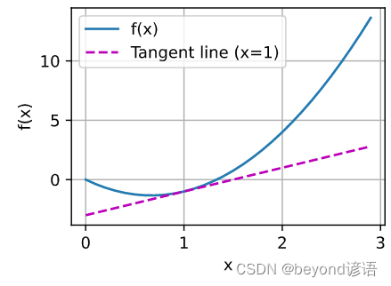
绘制函数u = f(x)及其在x = 1处的切线y = 2x - 3,其中系数是切线的斜率
x = np.arange(0, 3, 0.1)
plot(x, [f(x), 2 * x - 3], 'x', 'f(x)', legend=['f(x)', 'Tangent line (x=1)'])
二、自动微分
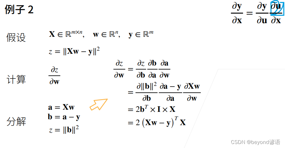
1,定义函数y = 2 (x^T) x,对列向量x求导
创建变量x并为其分配一个初始值
import torch

x = torch.arange(5.0)
x
"""
tensor([0., 1., 2., 3., 4.])
"""
存储梯度
x.requires_grad_(True)  # 等价于x=torch.arange(5.0,requires_grad=True)
x.grad  # 默认值是None    y对x求导的结果就存放在这里了
计算y
y = 2 * torch.dot(x, x) # 按元素乘法,然后进行求和来表示两个向量的点积(dot)
y # 2 * (0*0 + 1*1 + 2*2 + 3*3 + 4*4) = 2 * 30 = 60
"""
tensor(60., grad_fn=<MulBackward0>)
"""
调用反向传播函数来自动计算y关于x每个分量的梯度,并打印这些梯度
y.backward()
x.grad
"""
tensor([ 0.,  4.,  8., 12., 16.])
"""
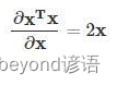
y = 2 (x^T) x关于x的梯度应为2 * 2x = 4x,进行验证
x.grad == 4 * x
"""
tensor([True, True, True, True, True])
"""
2,对函数y = x.sum()求导
在默认情况下,PyTorch会累积梯度,需要清除之前的值
x.grad.zero_()
求向量的sum,梯度为全1
y = x.sum()
y.backward()
x.grad
"""
tensor([1., 1., 1., 1., 1.])
"""
3,非标量变量的反向传播
创建变量x并为其分配一个初始值
import torch

x = torch.arange(5.0)
x.requires_grad_(True)  # 等价于x=torch.arange(5.0,requires_grad=True)
x.grad  # 默认值是None    y对x求导的结果就存放在这里了
当y不是标量时,向量y关于向量x的导数的最自然解释是一个矩阵
对于高阶和高维的y和x,求导的结果可以是一个高阶张量
# 对非标量调用backward需要传入一个gradient参数,该参数指定微分函数关于self的梯度。
# 求偏导数的和,所以传递一个1的梯度是合适的
#x.grad.zero_()
y = x * x
# 等价于y.backward(torch.ones(len(x)))
y.sum().backward() #标量 求导
x.grad
"""
tensor([0., 2., 4., 6., 8.])
"""
4,分离计算
分离计算即:将某些计算移动到记录的计算图之外,函数为:detach()
假设y是作为x的函数计算的,而z则是作为y和x的函数计算的
分离y来返回一个新变量u,该变量与y具有相同的值, 但丢弃计算图中如何计算y的任何信息
即:梯度不会向后流经u到x
反向传播函数计算z=ux关于x的偏导数,同时将u作为常数处理, 而不是z=xx*x关于x的偏导数
创建变量x并为其分配一个初始值
import torch

x = torch.arange(5.0)
x.requires_grad_(True)  # 等价于x=torch.arange(5.0,requires_grad=True)
x.grad  # 默认值是None    y对x求导的结果就存放在这里了
#x.grad.zero_()
y = x * x
u = y.detach()
z = u * x

z.sum().backward()
x.grad == u
"""
tensor([True, True, True, True, True])
"""
由于记录了y的计算结果,可以随后在y上调用反向传播, 得到y=x*x关于的x的导数,即2 * x
x.grad.zero_()
y.sum().backward()
x.grad == 2 * x
"""
tensor([True, True, True, True, True])
"""
5, Python控制流的梯度计算
使用自动微分的一个好处是: 即使构建函数的计算图需要通过Python控制流(例如,条件、循环或任意函数调用),仍然可以计算得到的变量的梯度
while循环的迭代次数和if语句的结果都取决于输入a的值
def f(a):
    b = a * 2
    while b.norm() < 1000:
        b = b * 2
    if b.sum() > 0:
        c = b
    else:
        c = 100 * b
    return c
f函数输入a中是分段线性的,对于任何a,存在某个常量标量k,使得f(a)=k*a,其中k的值取决于输入a
a = torch.randn(size=(), requires_grad=True)
d = f(a)
d.backward()
故可以用d/a验证梯度是否正确
a.grad == d / a
"""
tensor(True)
"""