getwd()
dir.create("/home/data/t040413/silicosis/fibroblast_myofibroblast/monocle5.17")
setwd("/home/data/t040413/silicosis/fibroblast_myofibroblast/monocle5.17")
#数据太大转到Linux服务器处理
.libPaths(c("/home/data/refdir/Rlib/", "/home/data/t040413/R/x86_64-pc-linux-gnu-library/4.2", "/usr/local/lib/R/library"))
library(Seurat)
load("/home/data/t040413/silicosis/fibroblast_myofibroblast/subset_data_fibroblast_myofibroblast.rds")
DotPlot(subset_data,features = c("Inmt","Gpx3","Fn1","Acta2","Serpinf1","Pi16",
"Col15a","Adamdec1","Npnt","Fbln1","Bmp4",
'Lrrc15',"Hhip","Comp",
"Cxcl15","Cxcl12","Ccl19"))+RotatedAxis()
#BiocManager::install("monocle",force = TRUE)
#library(monocle)
#devtools::load_all("/home/data/t040413/R/yll/usr/local/lib/R/site-library/monocle/")
#library(monocle)
DimPlot(subset_data,label = T)
head([email protected])
subset_data$cell.type=subset_data$seurat_clusters
Idents(subset_data)=subset_data$seurat_clusters #subset_data$cell.type
#Idents(subset_data)=subset_data$Idents.subset_data.
table(Idents(subset_data))
DefaultAssay(subset_data)
new.metadata <- merge([email protected],
data.frame(Idents(subset_data)),
by = "row.names",sort = FALSE)
head(new.metadata)
rownames(new.metadata)<-new.metadata[,1]
head([email protected])
identical(rownames(new.metadata),rownames([email protected]))
[email protected]<-new.metadata
table(subset_data$cell.type,Idents(subset_data))
head(subset_data)
expression_matrix <- as(as.matrix(subset_data@assays$RNA@counts), 'sparseMatrix')
head(expression_matrix)
identical(colnames(expression_matrix),rownames(new.metadata))
devtools::load_all("/home/data/t040413/ipf/diseased_lung_covid20/monocle/")
library(Seurat)
head([email protected])
cell_metadata <- new('AnnotatedDataFrame',[email protected])
head([email protected])
head(cell_metadata)
gene_annotation <- new('AnnotatedDataFrame',data=data.frame(gene_short_name = row.names(subset_data),
row.names = row.names(subset_data)))
head(gene_annotation)
fData(gene_annotation)
length(Idents(subset_data))
DimPlot(subset_data,group.by = "cell.type",label = T)
DimPlot(subset_data,label = T)
monocle_cds <- monocle::newCellDataSet(expression_matrix,
phenoData = cell_metadata,
featureData = gene_annotation,
lowerDetectionLimit = 0.5,
expressionFamily = negbinomial.size())
###################################################################################
##归一化######
cds <- monocle_cds
cds <- estimateSizeFactors(cds)
cds <- estimateDispersions(cds) ## Removing 110 outliers #下面的cell.type 为subset_Data 的meta信息
#library("BiocGenerics")#并行计算
#devtools::load_all("/home/data/t040413/ipf/diseased_lung_covid20/monocle/")
#https://www.jianshu.com/p/5d6fd4561bc0#
diff_test_res <- differentialGeneTest(cds,fullModelFormulaStr = "~ cell.type")
pData(cds)
deg=subset(diff_test_res,qval<0.01)
deg=deg[order(deg$qval,decreasing = T),]
head(deg)
ordergene=rownames(deg)
pdf("train.ordergenes.pdf")
plot_ordering_genes(cds)
dev.off()
length(ordergene)
### inference the pseudotrajectory###########################################################################################
# step1: select genes for orderding setOrderingFilter() #
ordering_genes <- row.names (subset(diff_test_res, qval < 0.01))
length(ordering_genes)# 6354
cds <- setOrderingFilter(cds, ordering_genes)
# step2: dimension reduction=> reduceDimension() DDRTree #
cds <- reduceDimension(cds, max_components = 2,method = 'DDRTree')
#source("./order_cells.R")
#unloadNamespace('monocle')
#devtools::load_all("../monocle_2.26.0 (1).tar/monocle_2.26.0 (1)/monocle/")
#devtools::load_all("/home/data/t040413/ipf/diseased_lung_covid20/monocle/")
cds <- orderCells(cds)
getwd()
save(diff_test_res,cds,
subset_data,file = "/home/data/t040413/silicosis/fibroblast_myofibroblast/monocle5.17/cds_noyet_root_diff_genes.Rdata")
devtools::load_all("/home/data/t040413/ipf/diseased_lung_covid20/monocle/")
load("/home/data/t040413/silicosis/fibroblast_myofibroblast/monocle5.17/cds_noyet_root_diff_genes.Rdata")
pData(cds)
deg=subset(diff_test_res,qval<0.01)
deg=deg[order(deg$qval,decreasing = T),]
head(deg)
ordergene=rownames(deg)
1#根据cds@phenoData@data信息上色
pdf("1.pseudutime.cell.type.pre.order.pdf")
plot_cell_trajectory(cds, color_by = "cell.type")
dev.off()
pdf("1.pseudutime.stim.pre.order.pdf")
plot_cell_trajectory(cds, color_by = "stim")
dev.off()
pdf("1.pseudutime.State.pre.order.pdf")
plot_cell_trajectory(cds, color_by = "State")
dev.off()
###### split ########
pdf("2.split.pseudutime.Seurat.cell.type.pdf")
plot_cell_trajectory(cds, color_by = 'cell.type') + facet_wrap(~cell.type)
dev.off()
pdf("2.split.pseudutime.stim.pdf")
plot_cell_trajectory(cds, color_by = "stim") + facet_wrap(~stim)
dev.off()
#https://www.jianshu.com/p/5d6fd4561bc0
pdf("4.split.pseudutime.Seurat.State.pdf")
plot_cell_trajectory(cds, color_by = 'cell.type') + facet_wrap(~State)
dev.off()
pdf("3.split.pseudutime.Seurat.cell.type_State.pdf")
plot_cell_trajectory(cds, color_by = 'State') + facet_wrap(~cell.type)
dev.off()
getwd()
table(pData(cds)$State,pData(cds)$cell.type)
openxlsx::write.xlsx(table(pData(cds)$State,pData(cds)$cell.type), "State_cellType_summary.xlsx", colnames=T, rownames=T)
table(pData(cds)$State,pData(cds)$stim)
openxlsx::write.xlsx(table(pData(cds)$State,pData(cds)$stim), "State_Stim_summary.xlsx", colnames=T, rownames=T)
##we set the state 2 as root ########state 2 with most cells in Endothelial cells
#这里设置谁为root??
DimPlot(subset_data,label = T)
table(Idents(subset_data))
DefaultAssay(subset_data)<-"RNA"
DimPlot(subset_data,label = T)
dev.off()
table(subset_data$cell.type)
getwd()
phenoData(cds) %>%varMetadata()
data(phenoData(cds))
View(phenoData(cds))
cds <- orderCells(cds,root_state=1)
pdf("4.pseudutime.Pseudotime.pdf")
p=plot_cell_trajectory(cds, color_by = "Pseudotime")
print(p)
dev.off()
2#沿着时间轴的细胞密度图
library(ggpubr)
df=pData(cds) #取出cds@phenoData@data内容
head(df)
ggplot(df,aes(x = Pseudotime,colour=cell.type,fill=cell.type))+
geom_density(bw=0.5,size=1,alpha=0.5)+
theme_classic2()
3#提取感兴趣的细胞进行可视化
#比如对状态7感兴趣
df=pData(cds)
cells_7=subset(df,State=="7") %>%rownames()
#保存拟时序分析表格
write.csv(df,file = "./pseudotime.csv")
4#可视化指定基因
4.1#可视化ordergene top5基因,并将其对象取出
keygenes=head(ordergene,5)
cds_subset=cds[keygenes,]
#可视化基因
plot_genes_in_pseudotime(cds_subset = cds_subset,color_by = "cell.type")
##可视化:以state/celltype/pseudotime进行
p1 <- plot_genes_in_pseudotime(cds_subset, color_by = "State")
p2 <- plot_genes_in_pseudotime(cds_subset, color_by = "cell.type")
p3 <- plot_genes_in_pseudotime(cds_subset, color_by = "Pseudotime")
plotc <- p1|p2|p3
plotc
ggsave("./Genes_pseudotimeplot.pdf",plot = plotc,width = 16,height = 8)
4.2#指定基因
s.genes=unique(c(
"Fn1", "Dcn", #"Fap",
"Fbln1", #"Ccl19",
# inflammatory 0
'Ccl6',"Il1b","Lyz2",
#ap 1
#'H2-Aa',"H2-Ab1","H2-Eb1",
# inflammatory??? 5
# "Pf4",
#inflamm grem1 7
"Grem1",
#universal fib 2
"Dpt","Serpinf1","Pi16","Cd34",
#specialized fib 3
"Selenbp1","Sod3", "Inmt","Gpx3","Npnt","Scube2","Wnt2","Vcam1",
# Hhip 4
"Hhip","Mgp",
#myo 6
"Acta2","Myh11",
#ccl21 8
"Ccl21a",
# acta 9
# Endothelial-like fib 10
"Egfl7"
#delete 11
)
)
plot_genes_jitter(cds[s.genes,],grouping = "State")
getwd()
ggsave(filename = "markersgene.pdf",width = 8,height = 100,limitsize = FALSE)
plot_genes_in_pseudotime(cds[s.genes,],color_by = "State")
ggsave(filename = "markersgene_genes_in_pseudotime.pdf",width = 8,height = 100,limitsize = FALSE)
5#拟时序展示单个基因表达变化
pData(cds)$Inmt=log2(exprs(cds)["Inmt",]+1)
plot_cell_trajectory(cds,color_by = "Inmt")
plot_cell_trajectory(cds,color_by = "Inmt")+scale_color_continuous()
pData(cds)$Serpinf1=log2(exprs(cds)["Serpinf1",]+1)
plot_cell_trajectory(cds,color_by = "Serpinf1")
plot_cell_trajectory(cds,color_by = "Serpinf1")+scale_color_continuous()
6#拟时差异基因热图
diff_test=diff_test_res
sig_gene_names <- row.names(subset(diff_test, qval < 1e-04))
p2 = plot_pseudotime_heatmap(cds[sig_gene_names,], num_clusters=5,
show_rownames=T, return_heatmap=T)
plot_pseudotime_heatmap(cds[s.genes,], num_clusters=5,
show_rownames=T, return_heatmap=T)
ggsave("pseudotime/pseudotime_heatmap2_selectedmarkergenes.png", width = 5, height = 130,
limitsize = FALSE)
6.1#把每个cluster的基因单独提取出来分析 某个亚群提取
p2$tree_row
p2$gtable
clusters=cutree(p2$tree_row,k=5)
clustering=data.frame(clusters)
head(clustering)
clustering[,1]=as.character(clustering[,1])
colnames(clustering)="Gene_Clusters"
table(clustering)
write.csv(clustering,file = "./time_gene_clustering_all.csv")
7#按照pseudotime来计算差异基因
diff_pseudotime_test_res <- differentialGeneTest(cds[s.genes,],
fullModelFormulaStr = "~ sm.ns(Pseudotime)")
plot_pseudotime_heatmap(cds[rownames(diff_pseudotime_test_res),],num_clusters=5,
show_rownames=T, return_heatmap=T)
diff_test_res %>%head()
8##分支点的分析
BEAM_res=BEAM(cds[ordergene[1:400],],branch_point = 1,cores =1,
progenitor_method='sequential_split') #progenitor_method = c('sequential_split', 'duplicate'),
BEAM_res=BEAM(cds[s.genes,],branch_point = 1,cores =1,
progenitor_method='sequential_split') #progenitor_method = c('sequential_split', 'duplicate'),
BEAM_res=BEAM(cds[rownames(subset(diff_test_res,qval<0.01)),],branch_point = 1,cores =1,
progenitor_method='sequential_split') #progenitor_method = c('sequential_split', 'duplicate'),
head(BEAM_res)
#会返回每个基因的显著性,显著的基因就是那些随不同branch变化的基因
#这一步很慢
BEAM_res=BEAM_res[,c("gene_short_name","pval","qval")]
head(BEAM_res)
dim(BEAM_res)
saveRDS(BEAM_res, file = "BEAM_res.rds")
col_sum=colSums(exprs(cds)[rownames(BEAM_res),])
col_sum
#https://zhuanlan.zhihu.com/p/378365295
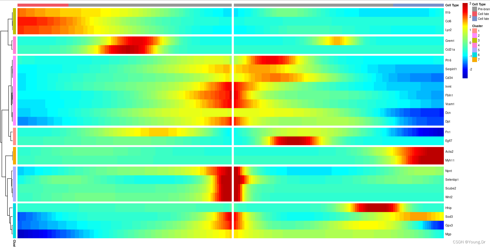
plot_genes_branched_heatmap(cds[rownames(BEAM_res),col_sum!=0],
branch_point = 1 ,#指定绘制的分支,
num_clusters = 7,
show_rownames = T) #是否返回一些重要信息
tmp1=plot_genes_branched_heatmap(cds[rownames(BEAM_res),col_sum!=0],
branch_point = 1 ,#指定绘制的分支,
num_clusters = 7,
show_rownames = T,
return_heatmap = T ) #是否返回一些重要信息
ggsave("beam_branched_heatmap.pdf",width = 7,height = 70,limitsize = FALSE)
pdf("branched_heatmap.pdf",width = 5,height = 6)
tmp1$ph_res
dev.off()
ls()
8.1#取出相应cluster的基因 差异基因按照热图结果排序并保存
#head(df) #https://zhuanlan.zhihu.com/p/378365295
#hp.genes=p$ph_res$tree_row$labels[p$ph_res$tree_row$order]
8.2##提取画图的细节信息
# Set the max.print option to a higher value
options(max.print = 99999)
sink("a.txt")
plot_genes_branched_heatmap(cds[rownames(BEAM_res),col_sum!=0],
branch_point = 1, num_clusters = 7,cores = 1,return_heatmap=TRUE)
dev.off()
sink()
sink(NULL)
# Check if the output is redirected
head(deg)
if (is.null(sink.number())) {
# Output is not redirected, proceed with printing
head(deg)
} else {
# Output is redirected, stop the redirection and print
sink(NULL)
head(deg)
}
a=read.table("./a.txt",sep = "\t")
8.3 #富集分析
gene_group=tmp1$annotation_row
gene_group$gene=rownames(gene_group)
library(clusterProfiler)
library(org.Hs.eg.db)
allcluster_go=data.frame()
for (i in unique(gene_group$Cluster)) {
small_gene_group=filter(gene_group,gene_group$Cluster==i)
df_name=bitr(small_gene_group$gene, fromType="SYMBOL", toType=c("ENTREZID"), OrgDb="org.Hs.eg.db")
go <- enrichGO(gene = unique(df_name$ENTREZID),
OrgDb = org.Hs.eg.db,
keyType = 'ENTREZID',
ont = "BP",
pAdjustMethod = "BH",
pvalueCutoff = 0.05,
qvalueCutoff = 0.2,
readable = TRUE)
go_res=go@result
if (dim(go_res)[1] != 0) {
go_res$cluster=i
allcluster_go=rbind(allcluster_go,go_res)
}
}
head(allcluster_go[,c("ID","Description","qvalue","cluster")])
getwd()
#############https://cloud.tencent.com/developer/article/1692225
#################################3
#Once we have a trajectory, we can use differentialGeneTest() to find genes
#that have an expression pattern that varies according to pseudotime.
getwd()
FeaturePlot(subset_data,features = "Inmt",split.by = "stim",label = T)
pdf("/home/data/t040413/silicosis/fibroblast_myofibroblast/2_featureplot_clusters_Split_Inmt.pdf",width = 19,height = 5)
p=FeaturePlot(subset_data,features = "Inmt",split.by = "stim",label = T)
print(p)
dev.off()
plot_pseudotime_heatmap(cds[c('CX3CR1',"SPP1"),],
num_clusters = 5,
# cores = 4,
show_rownames = T)
###########################cds 里面的内容
fData(cds) %>%head()
pData(cds) %>%head()
subset(fData(cds),
gene_short_name %in% c("TPM1", "MYH3", "CCNB2", "GAPDH"))
colours=seq(1,12,1)
p1=plot_cell_trajectory(cds,x=1,y=2,color_by = "cell.type")+
theme(legend.position = "none",panel.border = element_blank())+#第一个legennd去掉
scale_color_manual(values =colours ) #colours()
p2=plot_complex_cell_trajectory(cds,x=1,y = 2,
color_by = "cell.type")+
scale_color_manual(values = colours)+ #colours()
theme(legend.title = element_blank())
p1|p2
#############感兴趣基因的变化图
head([email protected])
plot_genes_jitter(cds[c("TPM1", "MYH3", "CCNB2", "GAPDH"),],
grouping = "cell.type", color_by = "cell.type", plot_trend = TRUE) +
facet_wrap( ~ feature_label, scales= "free_y")
#######拟时序热图
sig_gene_names=markers_for_eachcluster %>%
group_by(cluster) %>% top_n(n = 5,wt = avg_log2FC) %>% ##加不加引号区别很大
select(gene) %>% ungroup() %>%
pull(gene)
getwd()
p1 = plot_pseudotime_heatmap(cds[sig_gene_names,], num_clusters=3,
show_rownames=T, return_heatmap=T)
ggsave("pseudotime/pseudotime_heatmap1.png", plot = p1, width = 5, height = 8)
################################################################################
#https://davetang.org/muse/2017/10/01/getting-started-monocle/