2023年的深度学习入门指南(11) - Triton

上一篇我们学习了如何用CUDA进行编程。
下面我们将介绍几种深度学习GPU编程的优化方法。

第一种我们称之为多面体编译器。我们知道，在传统的IR，比如LLVM-IR中，使用条件分支来编码控制流信息。这种相对较低级的格式使得静态分析输入程序的运行时行为（例如缓存未命中）并通过使用平铺、融合和交换来自动优化循环变得困难。为了解决这个问题，多面体编译器依赖于具有静态可预测控制流的程序表示，从而实现对数据局部性和并行性的强大的编译时程序变换。比如最近很火的MLIR就是这样的技术。

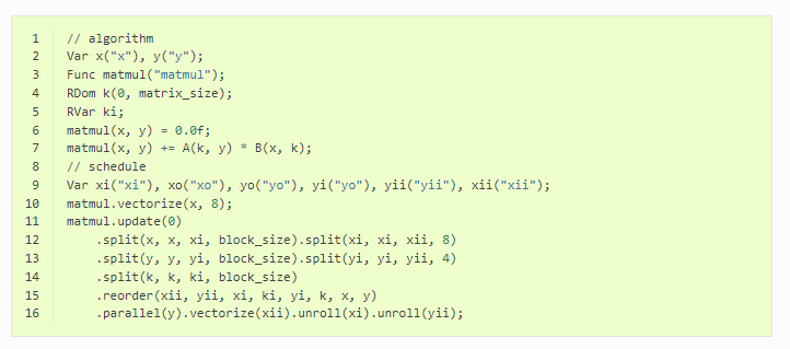
第二种叫做调度语言。这方面最流行的系统是TVM，它提供了跨广泛平台的良好性能以及内置的自动调度机制。分层原则是计算机科学中一个众所周知的设计原则：程序应该分解成模块化的抽象层，将其算法的语义与其实现的细节分开。像Halide和TVM这样的系统将这种理念推到了语法层面，通过使用调度语言在语法层面上强制实现这种分离。这种方法的好处在矩阵乘法的情况下尤其明显，如下所示，算法的定义（第1-7行）与其实现（第8-16行）是完全独立的，这意味着两者可以独立维护、优化和分发。

第三种就是Triton，Triton编译器大量使用块级数据流分析技术，该技术基于目标程序的控制流和数据流结构静态地调度迭代块。

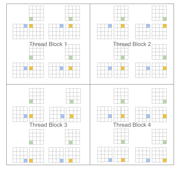
上篇我们花了不少精力算线程块，其实就是让大家理解，CUDA的线程在线程块中可能是很分散的：

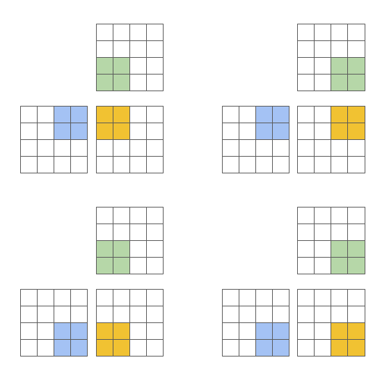
而Triton希望能够让它们更有组织一些：

为了解决这个问题，Triton编译器能够自动地应用很多种优化，例如自动合并、线程重组、预取、自动向量化、张量核心感知的指令选择、共享内存分配/同步、异步复制调度。

用Triton写核函数

我们先来看一下Triton的核函数是什么样子的：

@triton.jit
def add_kernel(
    x_ptr,  # *Pointer* to first input vector.
    y_ptr,  # *Pointer* to second input vector.
    output_ptr,  # *Pointer* to output vector.
    n_elements,  # Size of the vector.
    BLOCK_SIZE: tl.constexpr,  # Number of elements each program should process.
                 # NOTE: `constexpr` so it can be used as a shape value.
):
    # There are multiple 'programs' processing different data. We identify which program
    # we are here:
    pid = tl.program_id(axis=0)  # We use a 1D launch grid so axis is 0.
    # This program will process inputs that are offset from the initial data.
    # For instance, if you had a vector of length 256 and block_size of 64, the programs
    # would each access the elements [0:64, 64:128, 128:192, 192:256].
    # Note that offsets is a list of pointers:
    block_start = pid * BLOCK_SIZE
    offsets = block_start + tl.arange(0, BLOCK_SIZE)
    # Create a mask to guard memory operations against out-of-bounds accesses.
    mask = offsets < n_elements
    # Load x and y from DRAM, masking out any extra elements in case the input is not a
    # multiple of the block size.
    x = tl.load(x_ptr + offsets, mask=mask)
    y = tl.load(y_ptr + offsets, mask=mask)
    output = x + y
    # Write x + y back to DRAM.
    tl.store(output_ptr + offsets, output, mask=mask)

可以看到，跟我们之前写的CUDA代码似曾相识，只不过是cudaMemcpy之类的操作被封装了。

@triton.jit
def add_kernel(
    x_ptr,  # *Pointer* to first input vector.
    y_ptr,  # *Pointer* to second input vector.
    output_ptr,  # *Pointer* to output vector.
    n_elements,  # Size of the vector.
    BLOCK_SIZE: tl.constexpr,  # Number of elements each program should process.
                 # NOTE: `constexpr` so it can be used as a shape value.
):

@triton.jit: 这是一个Python装饰器，表示它是一个Triton内核函数,将由Triton编译器编译为GPU代码。
定义一个函数add_kernel，该函数接受四个参数：指向第一个输入向量的指针x_ptr、指向第二个输入向量的指针y_ptr、指向输出向量的指针output_ptr以及输入向量的大小n_elements。
BLOCK_SIZE: tl.constexpr: 定义一个常量BLOCK_SIZE，它表示每个线程块处理的元素个数，它的类型是tl.constexpr，表示它可以用作静态形状值。

pid = tl.program_id(axis=0) 

获取当前程序所在的线程块ID。

block_start = pid * BLOCK_SIZE: 计算当前线程块处理的第一个元素的位置。

offsets = block_start + tl.arange(0, BLOCK_SIZE): 计算每个线程处理的元素位置。

mask = offsets < n_elements: 创建一个布尔掩码，用于过滤超出输入向量范围的元素。

x = tl.load(x_ptr + offsets, mask=mask): 从输入向量x中加载数据。

y = tl.load(y_ptr + offsets, mask=mask): 从输入向量y中加载数据。

output = x + y: 将x和y相加。

tl.store(output_ptr + offsets, output, mask=mask): 将结果写回到输出向量中。

操作都比较基本，就不多作解释了。

总结一下上面代码用到的Triton特性：

• @triton.jit装饰器，用于将Python函数编译成GPU可执行的内核函数。
• tl.program_id函数，用于获取当前程序（或线程）的唯一索引，范围从0到总程序数减1。
• tl.grid_size函数，用于获取总程序数，等于启动内核时指定的块数乘以每块的线程数。
• tl.constexpr类型，用于声明一个常量表达式参数，可以在编译时确定其值，并用于指定数组或张量的形状。
• tl.arange函数，用于创建一个从0到指定值的连续整数序列，类似于Python中的range函数。
• tl.load函数，用于从全局内存中加载数据到寄存器中，可以指定一个偏移量和一个掩码。
• tl.store函数，用于将数据从寄存器中存储到全局内存中，可以指定一个偏移量和一个掩码。

这段代码的逻辑是这样的：

• 首先，根据当前程序的索引和每个程序应该处理的元素数（即块大小），计算出输入向量中的起始位置。
• 然后，根据起始位置和块大小，创建一个偏移量数组，表示每个程序要访问的输入元素的索引。
• 接着，创建一个掩码数组，用于过滤掉超出输入向量长度的偏移量。
• 然后，根据偏移量和掩码，从输入指针中加载x和y的元素到寄存器中，并计算它们的和。
• 最后，根据偏移量和掩码，将计算结果从寄存器中存储到输出指针中。

这样，每个程序都可以并行地处理一部分输入向量，并将结果写入输出向量中。这种方式可以提高内存访问的效率和并行度。

def add(x: torch.Tensor, y: torch.Tensor):
    # We need to preallocate the output.
    output = torch.empty_like(x)
    assert x.is_cuda and y.is_cuda and output.is_cuda
    n_elements = output.numel()
    # The SPMD launch grid denotes the number of kernel instances that run in parallel.
    # It is analogous to CUDA launch grids. It can be either Tuple[int], or Callable(metaparameters) -> Tuple[int].
    # In this case, we use a 1D grid where the size is the number of blocks:
    grid = lambda meta: (triton.cdiv(n_elements, meta['BLOCK_SIZE']),)
    # NOTE:
    #  - Each torch.tensor object is implicitly converted into a pointer to its first element.
    #  - `triton.jit`'ed functions can be indexed with a launch grid to obtain a callable GPU kernel.
    #  - Don't forget to pass meta-parameters as keywords arguments.
    add_kernel[grid](x, y, output, n_elements, BLOCK_SIZE=1024)
    # We return a handle to z but, since `torch.cuda.synchronize()` hasn't been called, the kernel is still
    # running asynchronously at this point.
    return output

上面这段代码主要就做了一件事，就是计算线程网格的合适大小，然后调用核函数。

torch.manual_seed(0)
size = 98432
x = torch.rand(size, device='cuda')
y = torch.rand(size, device='cuda')
output_torch = x + y
output_triton = add(x, y)
print(output_torch)
print(output_triton)
print(
    f'The maximum difference between torch and triton is '
    f'{
      
      torch.max(torch.abs(output_torch - output_triton))}'
)

然后我们就用Triton的核函数与PyTorch的计算做一个对比，看看谁快。

tensor([1.3713, 1.3076, 0.4940,  ..., 1.3374, 1.4960, 0.9115], device='cuda:0')
tensor([1.3713, 1.3076, 0.4940,  ..., 1.3374, 1.4960, 0.9115], device='cuda:0')
The maximum difference between torch and triton is 0.0

在我的电脑上两者反正差不多。

求softmax的例子

我们再来看一个Triton的例子，求softmax.

还是先是核函数：

@triton.jit
def softmax_kernel(
    output_ptr, input_ptr, input_row_stride, output_row_stride, n_cols,
    BLOCK_SIZE: tl.constexpr
):
    # The rows of the softmax are independent, so we parallelize across those
    row_idx = tl.program_id(0)
    # The stride represents how much we need to increase the pointer to advance 1 row
    row_start_ptr = input_ptr + row_idx * input_row_stride
    # The block size is the next power of two greater than n_cols, so we can fit each
    # row in a single block
    col_offsets = tl.arange(0, BLOCK_SIZE)
    input_ptrs = row_start_ptr + col_offsets
    # Load the row into SRAM, using a mask since BLOCK_SIZE may be > than n_cols
    row = tl.load(input_ptrs, mask=col_offsets < n_cols, other=-float('inf'))
    # Subtract maximum for numerical stability
    row_minus_max = row - tl.max(row, axis=0)
    # Note that exponentiation in Triton is fast but approximate (i.e., think __expf in CUDA)
    numerator = tl.exp(row_minus_max)
    denominator = tl.sum(numerator, axis=0)
    softmax_output = numerator / denominator
    # Write back output to DRAM
    output_row_start_ptr = output_ptr + row_idx * output_row_stride
    output_ptrs = output_row_start_ptr + col_offsets
    tl.store(output_ptrs, softmax_output, mask=col_offsets < n_cols)

• @triton.jit装饰器，用于将Python函数编译成GPU可执行的内核函数。
• tl.program_id函数，用于获取当前程序（或线程）的唯一索引，范围从0到总程序数减1。
• tl.constexpr类型，用于声明一个常量表达式参数，可以在编译时确定其值，并用于指定数组或张量的形状。
• tl.arange函数，用于创建一个从0到指定值的连续整数序列，类似于Python中的range函数。
• tl.load函数，用于从全局内存中加载数据到寄存器中，可以指定一个偏移量和一个掩码。
• tl.max函数，用于计算一个张量在给定轴上的最大值。
• tl.exp函数，用于计算一个张量的指数函数，类似于Python中的math.exp函数。注意这个函数是快速但近似的（类似于CUDA中的__expf函数）。
• tl.sum函数，用于计算一个张量在给定轴上的求和。
• tl.store函数，用于将数据从寄存器中存储到全局内存中，可以指定一个偏移量和一个掩码。

这段代码的逻辑是这样的：

• 首先，根据当前程序的索引和输入矩阵的行跨度（即每行占用的字节数），计算出输入矩阵中当前行的起始指针。
• 然后，根据块大小（即每个程序处理的列数），创建一个偏移量数组，表示每个程序要访问的输入元素的索引。注意块大小是大于等于列数的最小2的幂，所以可以保证每行可以被一个块完全处理。
• 接着，根据偏移量和掩码（用于过滤掉超出列数的偏移量），从输入指针中加载当前行的元素到寄存器中，并减去当前行的最大值，以提高数值稳定性。
• 然后，对减去最大值后的元素进行指数运算，并在给定轴上求和，得到分母。然后将分子除以分母，得到softmax输出。
• 最后，根据偏移量和掩码（用于过滤掉超出列数的偏移量），将softmax输出从寄存器中存储到输出指针中。

这样，每个程序都可以并行地处理输入矩阵的一部分，并将结果写入输出矩阵中。这种方式可以提高内存访问和计算的效率和并行度。

然后第二步，我们还是计算该用多少线程。

def softmax(x):
    n_rows, n_cols = x.shape
    # The block size is the smallest power of two greater than the number of columns in `x`
    BLOCK_SIZE = triton.next_power_of_2(n_cols)
    # Another trick we can use is to ask the compiler to use more threads per row by
    # increasing the number of warps (`num_warps`) over which each row is distributed.
    # You will see in the next tutorial how to auto-tune this value in a more natural
    # way so you don't have to come up with manual heuristics yourself.
    num_warps = 4
    if BLOCK_SIZE >= 2048:
        num_warps = 8
    if BLOCK_SIZE >= 4096:
        num_warps = 16
    # Allocate output
    y = torch.empty_like(x)
    # Enqueue kernel. The 1D launch grid is simple: we have one kernel instance per row o
    # f the input matrix
    softmax_kernel[(n_rows,)](
        y,
        x,
        x.stride(0),
        y.stride(0),
        n_cols,
        num_warps=num_warps,
        BLOCK_SIZE=BLOCK_SIZE,
    )
    return y

其中输入矩阵 x 的形状为 (n_rows, n_cols)，表示有 n_rows 个行和 n_cols 个列。首先通过 triton.next_power_of_2(n_cols) 函数求出大于等于 n_cols 的最小的 2 的幂，作为块大小 BLOCK_SIZE。然后，根据 BLOCK_SIZE 的大小确定每个行使用的线程块数 num_warps。根据经验，当 BLOCK_SIZE 大于等于 2048 时，num_warps 设置为 8，当 BLOCK_SIZE 大于等于 4096 时，设置为 16。接着，为输出矩阵 y 分配与 x 相同的空间。最后，通过 softmax_kernel 函数计算 softmax，并将结果保存在 y 中。注意，softmax_kernel 函数接受的参数包括输入和输出矩阵指针、输入和输出矩阵行跨度、矩阵列数、线程块大小和行使用的线程块数。

然后我们跟PyTorch的比一下：

@torch.jit.script
def naive_softmax(x):
    """Compute row-wise softmax of X using native pytorch

    We subtract the maximum element in order to avoid overflows. Softmax is invariant to
    this shift.
    """
    # read  MN elements ; write M  elements
    x_max = x.max(dim=1)[0]
    # read MN + M elements ; write MN elements
    z = x - x_max[:, None]
    # read  MN elements ; write MN elements
    numerator = torch.exp(z)
    # read  MN elements ; write M  elements
    denominator = numerator.sum(dim=1)
    # read MN + M elements ; write MN elements
    ret = numerator / denominator[:, None]
    # in total: read 5MN + 2M elements ; wrote 3MN + 2M elements
    return ret

最后对比下结果是不是一样：

torch.manual_seed(0)
x = torch.randn(1823, 781, device='cuda')
y_triton = softmax(x)
y_torch = torch.softmax(x, axis=1)
assert torch.allclose(y_triton, y_torch), (y_triton, y_torch)

计算注意力

下面我们结合之前学习的自注意力的知识，用Triton来写个注意力模型：

@triton.jit
def _fwd_kernel(
    Q, K, V, sm_scale,
    L, M,
    Out,
    stride_qz, stride_qh, stride_qm, stride_qk,
    stride_kz, stride_kh, stride_kn, stride_kk,
    stride_vz, stride_vh, stride_vk, stride_vn,
    stride_oz, stride_oh, stride_om, stride_on,
    Z, H, N_CTX,
    BLOCK_M: tl.constexpr, BLOCK_DMODEL: tl.constexpr,
    BLOCK_N: tl.constexpr,
):
    start_m = tl.program_id(0)
    off_hz = tl.program_id(1)
    # initialize offsets
    offs_m = start_m * BLOCK_M + tl.arange(0, BLOCK_M)
    offs_n = tl.arange(0, BLOCK_N)
    offs_d = tl.arange(0, BLOCK_DMODEL)
    off_q = off_hz * stride_qh + offs_m[:, None] * stride_qm + offs_d[None, :] * stride_qk
    off_k = off_hz * stride_qh + offs_n[None, :] * stride_kn + offs_d[:, None] * stride_kk
    off_v = off_hz * stride_qh + offs_n[:, None] * stride_qm + offs_d[None, :] * stride_qk
    # Initialize pointers to Q, K, V
    q_ptrs = Q + off_q
    k_ptrs = K + off_k
    v_ptrs = V + off_v
    # initialize pointer to m and l
    m_prev = tl.zeros([BLOCK_M], dtype=tl.float32) - float("inf")
    l_prev = tl.zeros([BLOCK_M], dtype=tl.float32)
    acc = tl.zeros([BLOCK_M, BLOCK_DMODEL], dtype=tl.float32)
    # load q: it will stay in SRAM throughout
    q = tl.load(q_ptrs)
    # loop over k, v and update accumulator
    for start_n in range(0, (start_m + 1) * BLOCK_M, BLOCK_N):
        # -- compute qk ----
        k = tl.load(k_ptrs)
        qk = tl.zeros([BLOCK_M, BLOCK_N], dtype=tl.float32)
        qk += tl.dot(q, k)
        qk *= sm_scale
        qk = tl.where(offs_m[:, None] >= (start_n + offs_n[None, :]), qk, float("-inf"))
        # compute new m
        m_curr = tl.maximum(tl.max(qk, 1), m_prev)
        # correct old l
        l_prev *= tl.exp(m_prev - m_curr)
        # attention weights
        p = tl.exp(qk - m_curr[:, None])
        l_curr = tl.sum(p, 1) + l_prev
        # rescale operands of matmuls
        l_rcp = 1. / l_curr
        p *= l_rcp[:, None]
        acc *= (l_prev * l_rcp)[:, None]
        # update acc
        p = p.to(Q.dtype.element_ty)
        v = tl.load(v_ptrs)
        acc += tl.dot(p, v)
        # update m_i and l_i
        l_prev = l_curr
        m_prev = m_curr
        # update pointers
        k_ptrs += BLOCK_N * stride_kn
        v_ptrs += BLOCK_N * stride_vk
    # rematerialize offsets to save registers
    start_m = tl.program_id(0)
    offs_m = start_m * BLOCK_M + tl.arange(0, BLOCK_M)
    # write back l and m
    l_ptrs = L + off_hz * N_CTX + offs_m
    m_ptrs = M + off_hz * N_CTX + offs_m
    tl.store(l_ptrs, l_prev)
    tl.store(m_ptrs, m_prev)
    # initialize pointers to output
    offs_n = tl.arange(0, BLOCK_DMODEL)
    off_o = off_hz * stride_oh + offs_m[:, None] * stride_om + offs_n[None, :] * stride_on
    out_ptrs = Out + off_o
    tl.store(out_ptrs, acc)

代码是Triton中的一个内核函数，用于将一个批次的输入Q、K、V矩阵与权重矩阵相乘，然后执行 softmax 操作。具体来说，此内核函数通过计算每个位置的加权和，并将其存储在输出矩阵中来实现self-attention操作。在计算期间，每个线程块处理一个输入矩阵行的一部分，并将其存储在共享内存中，以便在处理其他行时可以重用该数据。

它的功能是根据输入的查询矩阵Q、键矩阵K和值矩阵V，计算输出矩阵Out，其中Out[i,j,:]是Q[i,:]和V[j,:]的加权平均，权重由Q[i,:]和K[j,:]的点积决定。它使用了以下的Triton特性：

• tl.arange函数，用于创建一个从0到指定值的连续整数序列，类似于Python中的range函数。
• tl.zeros函数，用于创建一个给定形状和类型的全零张量。
• tl.dot函数，用于计算两个张量的点积。
• tl.where函数，用于根据一个条件张量选择两个输入张量中的元素。
• tl.maximum函数，用于计算两个张量在给定轴上的最大值。
• tl.max函数，用于计算一个张量在给定轴上的最大值。
• tl.exp函数，用于计算一个张量的指数函数，类似于Python中的math.exp函数。注意这个函数是快速但近似的（类似于CUDA中的__expf函数）。
• tl.sum函数，用于计算一个张量在给定轴上的求和。

再看下一段：

@triton.jit
def _bwd_preprocess(
    Out, DO, L,
    NewDO, Delta,
    BLOCK_M: tl.constexpr, D_HEAD: tl.constexpr,
):
    off_m = tl.program_id(0) * BLOCK_M + tl.arange(0, BLOCK_M)
    off_n = tl.arange(0, D_HEAD)
    # load
    o = tl.load(Out + off_m[:, None] * D_HEAD + off_n[None, :]).to(tl.float32)
    do = tl.load(DO + off_m[:, None] * D_HEAD + off_n[None, :]).to(tl.float32)
    denom = tl.load(L + off_m).to(tl.float32)
    # compute
    do = do / denom[:, None]
    delta = tl.sum(o * do, axis=1)
    # write-back
    tl.store(NewDO + off_m[:, None] * D_HEAD + off_n[None, :], do)
    tl.store(Delta + off_m, delta)

这段代码定义了一个在反向传播中用到的 Triton 函数 _bwd_preprocess，它将 Out（前向传播的输出）、DO（当前反向传播的梯度值）和 L（前向传播中的标量指数）作为输入。BLOCK_M 是 Triton 的常量，表示每个 Triton 线程处理的条目数，D_HEAD 是另一个 Triton 常量，表示 Q/K/V 的头的维度。

函数的作用是执行一些预处理步骤，以便在后续的反向传播计算中使用。具体来说，它首先加载了 Out、DO 和 L 中的值，然后根据 L 中的标量指数计算了 do（即 $d^{\mathrm{out}}i/{\sum }_j\exp ({\mathrm{Out}}_{ij})$）。最后，函数计算了 ${\Delta }_i={\sum }_j{\mathrm{Out}}_{ij}\times d_{ij}^{\mathrm{out}}$，并将 do 和 Delta 的值存储到 NewDO 和 Delta 中。

最后我们看反向传播的部分：

@triton.jit
def _bwd_kernel(
    Q, K, V, sm_scale, Out, DO,
    DQ, DK, DV,
    L, M,
    D,
    stride_qz, stride_qh, stride_qm, stride_qk,
    stride_kz, stride_kh, stride_kn, stride_kk,
    stride_vz, stride_vh, stride_vk, stride_vn,
    Z, H, N_CTX,
    num_block,
    BLOCK_M: tl.constexpr, BLOCK_DMODEL: tl.constexpr,
    BLOCK_N: tl.constexpr,
):
    off_hz = tl.program_id(0)
    off_z = off_hz // H
    off_h = off_hz % H
    # offset pointers for batch/head
    Q += off_z * stride_qz + off_h * stride_qh
    K += off_z * stride_qz + off_h * stride_qh
    V += off_z * stride_qz + off_h * stride_qh
    DO += off_z * stride_qz + off_h * stride_qh
    DQ += off_z * stride_qz + off_h * stride_qh
    DK += off_z * stride_qz + off_h * stride_qh
    DV += off_z * stride_qz + off_h * stride_qh
    for start_n in range(0, num_block):
        lo = start_n * BLOCK_M
        # initialize row/col offsets
        offs_qm = lo + tl.arange(0, BLOCK_M)
        offs_n = start_n * BLOCK_M + tl.arange(0, BLOCK_M)
        offs_m = tl.arange(0, BLOCK_N)
        offs_k = tl.arange(0, BLOCK_DMODEL)
        # initialize pointers to value-like data
        q_ptrs = Q + (offs_qm[:, None] * stride_qm + offs_k[None, :] * stride_qk)
        k_ptrs = K + (offs_n[:, None] * stride_kn + offs_k[None, :] * stride_kk)
        v_ptrs = V + (offs_n[:, None] * stride_qm + offs_k[None, :] * stride_qk)
        do_ptrs = DO + (offs_qm[:, None] * stride_qm + offs_k[None, :] * stride_qk)
        dq_ptrs = DQ + (offs_qm[:, None] * stride_qm + offs_k[None, :] * stride_qk)
        # pointer to row-wise quantities in value-like data
        D_ptrs = D + off_hz * N_CTX
        m_ptrs = M + off_hz * N_CTX
        # initialize dv amd dk
        dv = tl.zeros([BLOCK_M, BLOCK_DMODEL], dtype=tl.float32)
        dk = tl.zeros([BLOCK_M, BLOCK_DMODEL], dtype=tl.float32)
        # k and v stay in SRAM throughout
        k = tl.load(k_ptrs)
        v = tl.load(v_ptrs)
        # loop over rows
        for start_m in range(lo, num_block * BLOCK_M, BLOCK_M):
            offs_m_curr = start_m + offs_m
            # load q, k, v, do on-chip
            q = tl.load(q_ptrs)
            # recompute p = softmax(qk, dim=-1).T
            # NOTE: `do` is pre-divided by `l`; no normalization here
            qk = tl.dot(q, tl.trans(k))
            qk = tl.where(offs_m_curr[:, None] >= (offs_n[None, :]), qk, float("-inf"))
            m = tl.load(m_ptrs + offs_m_curr)
            p = tl.exp(qk * sm_scale - m[:, None])
            # compute dv
            do = tl.load(do_ptrs)
            dv += tl.dot(tl.trans(p.to(Q.dtype.element_ty)), do)
            # compute dp = dot(v, do)
            Di = tl.load(D_ptrs + offs_m_curr)
            dp = tl.zeros([BLOCK_M, BLOCK_N], dtype=tl.float32) - Di[:, None]
            dp += tl.dot(do, tl.trans(v))
            # compute ds = p * (dp - delta[:, None])
            ds = p * dp * sm_scale
            # compute dk = dot(ds.T, q)
            dk += tl.dot(tl.trans(ds.to(Q.dtype.element_ty)), q)
            # compute dq
            dq = tl.load(dq_ptrs)
            dq += tl.dot(ds.to(Q.dtype.element_ty), k)
            tl.store(dq_ptrs, dq)
            # increment pointers
            dq_ptrs += BLOCK_M * stride_qm
            q_ptrs += BLOCK_M * stride_qm
            do_ptrs += BLOCK_M * stride_qm
        # write-back
        dv_ptrs = DV + (offs_n[:, None] * stride_qm + offs_k[None, :] * stride_qk)
        dk_ptrs = DK + (offs_n[:, None] * stride_kn + offs_k[None, :] * stride_kk)
        tl.store(dv_ptrs, dv)
        tl.store(dk_ptrs, dk)

这是实现Transformer网络中自注意力层的反向传播内核。它计算输入查询、键和值向量（dq、dk和dv）的梯度，给定输出张量（do）的梯度。在反向传播期间调用该内核以更新参数的梯度。

该内核在一个查询、键和值块上操作，其中每个块包含BLOCK_M个查询、BLOCK_M个键和BLOCK_N个值。计算在多个批次和头上并行进行，每个批次具有N_CTX个查询，每个头具有D_MODEL维度。

该函数以查询（Q）、键（K）、值（V）和输出梯度（DO）张量作为输入，以及softmax缩放因子（sm_scale）、块大小（BLOCK_M、BLOCK_N、BLOCK_DMODEL）和各种步幅等其他参数。它使用一系列矩阵乘法和约简计算来计算和更新输入张量（DQ、DK和DV）和其他辅助张量（L、M、D）的梯度。

最后，我们将其组合起来：

class _attention(torch.autograd.Function):

    @staticmethod
    def forward(ctx, q, k, v, sm_scale):
        BLOCK = 128
        # shape constraints
        Lq, Lk, Lv = q.shape[-1], k.shape[-1], v.shape[-1]
        assert Lq == Lk and Lk == Lv
        assert Lk in {
    
    16, 32, 64, 128}
        o = torch.empty_like(q)
        grid = (triton.cdiv(q.shape[2], BLOCK), q.shape[0] * q.shape[1], 1)
        L = torch.empty((q.shape[0] * q.shape[1], q.shape[2]), device=q.device, dtype=torch.float32)
        m = torch.empty((q.shape[0] * q.shape[1], q.shape[2]), device=q.device, dtype=torch.float32)
        num_warps = 4 if Lk <= 64 else 8

        _fwd_kernel[grid](
            q, k, v, sm_scale,
            L, m,
            o,
            q.stride(0), q.stride(1), q.stride(2), q.stride(3),
            k.stride(0), k.stride(1), k.stride(2), k.stride(3),
            v.stride(0), v.stride(1), v.stride(2), v.stride(3),
            o.stride(0), o.stride(1), o.stride(2), o.stride(3),
            q.shape[0], q.shape[1], q.shape[2],
            BLOCK_M=BLOCK, BLOCK_N=BLOCK,
            BLOCK_DMODEL=Lk, num_warps=num_warps,
            num_stages=2,
        )
        # print(h.asm["ttgir"])

        ctx.save_for_backward(q, k, v, o, L, m)
        ctx.grid = grid
        ctx.sm_scale = sm_scale
        ctx.BLOCK_DMODEL = Lk
        return o

    @staticmethod
    def backward(ctx, do):
        BLOCK = 128
        q, k, v, o, l, m = ctx.saved_tensors
        do = do.contiguous()
        dq = torch.zeros_like(q, dtype=torch.float32)
        dk = torch.empty_like(k)
        dv = torch.empty_like(v)
        do_scaled = torch.empty_like(do)
        delta = torch.empty_like(l)
        _bwd_preprocess[(ctx.grid[0] * ctx.grid[1], )](
            o, do, l,
            do_scaled, delta,
            BLOCK_M=BLOCK, D_HEAD=ctx.BLOCK_DMODEL,
        )
        _bwd_kernel[(ctx.grid[1],)](
            q, k, v, ctx.sm_scale,
            o, do_scaled,
            dq, dk, dv,
            l, m,
            delta,
            q.stride(0), q.stride(1), q.stride(2), q.stride(3),
            k.stride(0), k.stride(1), k.stride(2), k.stride(3),
            v.stride(0), v.stride(1), v.stride(2), v.stride(3),
            q.shape[0], q.shape[1], q.shape[2],
            ctx.grid[0],
            BLOCK_M=BLOCK, BLOCK_N=BLOCK,
            BLOCK_DMODEL=ctx.BLOCK_DMODEL, num_warps=8,
            num_stages=1,
        )
        # print(h.asm["ttgir"])
        return dq, dk, dv, None

在前向传播中，通过调用 _fwd_kernel 函数实现自注意力机制的计算，主要包含矩阵乘法和 Softmax 操作。其输入为 q, k, v 以及一个标量 sm_scale，输出为自注意力机制的结果 o。
在后向传播中，通过调用 _bwd_kernel 函数计算 q, k, v 的梯度。

Triton在量化中的应用

前面的两个例子都来自官方的样例。那么，在真实的大模型中，是否真的使用到了Triton呢。
答案是有的，在量化库bitsandbytes中就用到了Triton，我们看一个量化的片段：

    @triton.jit
    def _quantize_global(
        x_ptr,
        absmax_inv_ptr,
        output_ptr,
        n_elements,
        BLOCK_SIZE: tl.constexpr,
    ):
        pid = tl.program_id(axis=0)
        block_start = pid * BLOCK_SIZE
        offsets = block_start + tl.arange(0, BLOCK_SIZE)
        mask = offsets < n_elements
        x = tl.load(x_ptr + offsets, mask=mask)
        absmax_inv = tl.load(absmax_inv_ptr)
        output = tl.libdevice.llrint(127. * (x * absmax_inv))
        tl.store(output_ptr + offsets, output, mask=mask)

这段代码是用Triton语言编写的，用于实现全局量化的内核函数。它的功能是根据输入的浮点数数组x_ptr、最大绝对值的倒数absmax_inv_ptr和输出的整数数组output_ptr，将x_ptr中的每个元素乘以absmax_inv_ptr，然后四舍五入到最近的整数，并乘以127，得到量化后的结果。它使用了以下的Triton特性：

这里面新出现的是tl.libdevice.llrint函数，用于对一个浮点数进行四舍五入到最近的整数。

这段代码的逻辑是这样的：

• 首先，根据当前程序的索引和块大小（即每个程序处理的元素数），计算出输入和输出数组中要处理的元素的偏移量和掩码。掩码用于过滤掉超出数组长度的偏移量。
• 然后，从输入指针中加载要处理的元素x和最大绝对值的倒数absmax_inv到寄存器中。
• 接着，计算输出元素output，即将x乘以absmax_inv，然后四舍五入到最近的整数，并乘以127。
• 最后，将输出元素output从寄存器中存储到输出指针中。
  这样，每个程序都可以并行地处理输入和输出数组的一部分，并将结果写入输出数组中。这种方式可以提高内存访问和计算的效率和并行度。

然后再来一个计算线程网格的函数：

    def quantize_global(x: torch.Tensor):
        absmax = x.abs().max().unsqueeze(0)
        absmax_inv = 1./ absmax
        output = torch.empty(*x.shape, device='cuda', dtype=torch.int8)
        assert x.is_cuda and output.is_cuda
        n_elements = output.numel()
        grid = lambda meta: (triton.cdiv(n_elements, meta['BLOCK_SIZE']),)
        _quantize_global[grid](x, absmax_inv, output, n_elements)
        return output, 

小结

Triton也是Openai的产品，虽然还在演进之中，但是可以做为优化的一个选项。