AI实战训练营&MMDetection安装配置指南
一 MMDetection简介
 MMDetection 是被广泛使用的检测工具箱,包括了目标检测、实例分割、全景分割等多个通用检测方向,并支持了 75+ 个主流和前沿模型,为用户提供超过 440+ 个预训练模型,在学术研究和工业落地中拥有广泛应用。该框架的主要特点为:
- 模块化设计
MMDetection 将检测框架解耦成不同的模块组件,通过组合不同的模块组件,用户可以便捷地构建自定义的检测模型 - 支持多种检测任务
MMDetection 支持了各种不同的检测任务,包括目标检测,实例分割,全景分割,以及半监督目标检测。后续会重点支持多模态通用检测方向 - 速度快
基本的框和 mask 操作都实现了 GPU 版本,训练速度比其他代码库更快或者相当。 - 性能高
MMDetection 这个算法库源自于 COCO 2018 目标检测竞赛的冠军团队 MMDet 团队开发的代码,我们在之后持续进行了改进和提升。 新发布的 RTMDet 还在实时实例分割和旋转目标检测任务中取得了最先进的成果,同时也在目标检测模型中取得了最佳的的参数量和精度平衡。
版本迭代变化 2.0 - 3.0
在 MMDetection V2.0 基础上,通过更细粒度的模块解耦。进一步拆解出了数据、数据变换、模型、评测、可视化器等抽象,并将这些接口进行了统一设计,统一的数据流和细粒度的模块大幅提升了任务拓展性能。基于全新训练引擎 MMEngine 和计算机视觉的基础库 MMCV 进行了全面适配,经过对模型各个组件的重构和优化,全面提升了 MMDetection 的速度和精度,达到了现有检测框架中的最优水平。
MMDetection Repo: MMDetection Repo
MMDetection 官方文档链接:https://mmdetection.readthedocs.io/en/latest/
二 环境检测和安装
首先在jupyter中输入如下指令,当然也可以在终端输入,去掉前面的!号即可。可以打印出你本机的机器信息。
# Check nvcc version
!nvcc -V
# Check GCC version
!gcc --version

# 安装 mmengine 和 mmcv 依赖
# 为了防止后续版本变更导致的代码无法运行,我们暂时锁死版本
!pwd
%pip install -U "openmim"
!mim install "mmengine"
!mim install "mmcv"
# Install mmdetection
!rm -rf mmdetection
!git clone https://github.com/open-mmlab/mmdetection.git
%cd mmdetection
%pip install -e .
用这个代码可以打印出环境信息
from mmengine.utils import get_git_hash
from mmengine.utils.dl_utils import collect_env as collect_base_env

import mmdet

# 环境信息收集和打印
def collect_env():
    """Collect the information of the running environments."""
    env_info = collect_base_env()
    env_info['MMDetection'] = f'{

      mmdet.__version__}+{

      get_git_hash()[:7]}'
    return env_info


if __name__ == '__main__':
    for name, val in collect_env().items():
        print(f'{

      name}: {

      val}')

三 准备数据集
首先进入到我们MMDetection目录下,下载数据集。

准备好之后的数据会按照coco的格式

用下面的代码可以看到我们的数据,我们只看8张
import os
import matplotlib.pyplot as plt
from PIL import Image

%matplotlib inline
%config InlineBackend.figure_format = 'retina'

original_images = []
images = []
texts = []
plt.figure(figsize=(16, 5))

image_paths= [filename for filename in os.listdir('cat_dataset/images')][:8]

for i,filename in enumerate(image_paths):
    name = os.path.splitext(filename)[0]

    image = Image.open('cat_dataset/images/'+filename).convert("RGB")

    plt.subplot(2, 4, i+1)
    plt.imshow(image)
    plt.title(f"{

      filename}")
    plt.xticks([])
    plt.yticks([])

plt.tight_layout()

from pycocotools.coco import COCO
from PIL import Image
import numpy as np
import os.path as osp
import matplotlib.pyplot as plt
from matplotlib.collections import PatchCollection
from matplotlib.patches import Polygon

def apply_exif_orientation(image):
    _EXIF_ORIENT = 274
    if not hasattr(image, 'getexif'):
        return image

    try:
        exif = image.getexif()
    except Exception:
        exif = None

    if exif is None:
        return image

    orientation = exif.get(_EXIF_ORIENT)

    method = {


        2: Image.FLIP_LEFT_RIGHT,
        3: Image.ROTATE_180,
        4: Image.FLIP_TOP_BOTTOM,
        5: Image.TRANSPOSE,
        6: Image.ROTATE_270,
        7: Image.TRANSVERSE,
        8: Image.ROTATE_90,
    }.get(orientation)
    if method is not None:
        return image.transpose(method)
    return image


def show_bbox_only(coco, anns, show_label_bbox=True, is_filling=True):
    """Show bounding box of annotations Only."""
    if len(anns) == 0:
        return

    ax = plt.gca()
    ax.set_autoscale_on(False)

    image2color = dict()
    for cat in coco.getCatIds():
        image2color[cat] = (np.random.random((1, 3)) * 0.7 + 0.3).tolist()[0]

    polygons = []
    colors = []

    for ann in anns:
        color = image2color[ann['category_id']]
        bbox_x, bbox_y, bbox_w, bbox_h = ann['bbox']
        poly = [[bbox_x, bbox_y], [bbox_x, bbox_y + bbox_h],
                [bbox_x + bbox_w, bbox_y + bbox_h], [bbox_x + bbox_w, bbox_y]]
        polygons.append(Polygon(np.array(poly).reshape((4, 2))))
        colors.append(color)

        if show_label_bbox:
            label_bbox = dict(facecolor=color)
        else:
            label_bbox = None

        ax.text(
            bbox_x,
            bbox_y,
            '%s' % (coco.loadCats(ann['category_id'])[0]['name']),
            color='white',
            bbox=label_bbox)

    if is_filling:
        p = PatchCollection(
            polygons, facecolor=colors, linewidths=0, alpha=0.4)
        ax.add_collection(p)
    p = PatchCollection(
        polygons, facecolor='none', edgecolors=colors, linewidths=2)
    ax.add_collection(p)


coco = COCO('/gemini/code/mmdetection/cat_dataset/annotations/test.json')
image_ids = coco.getImgIds()
np.random.shuffle(image_ids)

plt.figure(figsize=(16, 5))

# 只可视化 8 张图片
for i in range(8):
    image_data = coco.loadImgs(image_ids[i])[0]
    image_path = osp.join('/gemini/code/mmdetection/cat_dataset/images/',image_data['file_name'])
    annotation_ids = coco.getAnnIds(
            imgIds=image_data['id'], catIds=[], iscrowd=0)
    annotations = coco.loadAnns(annotation_ids)

    ax = plt.subplot(2, 4, i+1)
    image = Image.open(image_path).convert("RGB")

    # 这行代码很关键,否则可能图片和标签对不上
    image=apply_exif_orientation(image)

    ax.imshow(image)

    show_bbox_only(coco, annotations)

    plt.title(f"{

      filename}")
    plt.xticks([])
    plt.yticks([])

plt.tight_layout()

四 自定义配置文件
本教程采用 RTMDet 进行演示,在开始自定义配置文件前,先来了解下 RTMDet 算法。
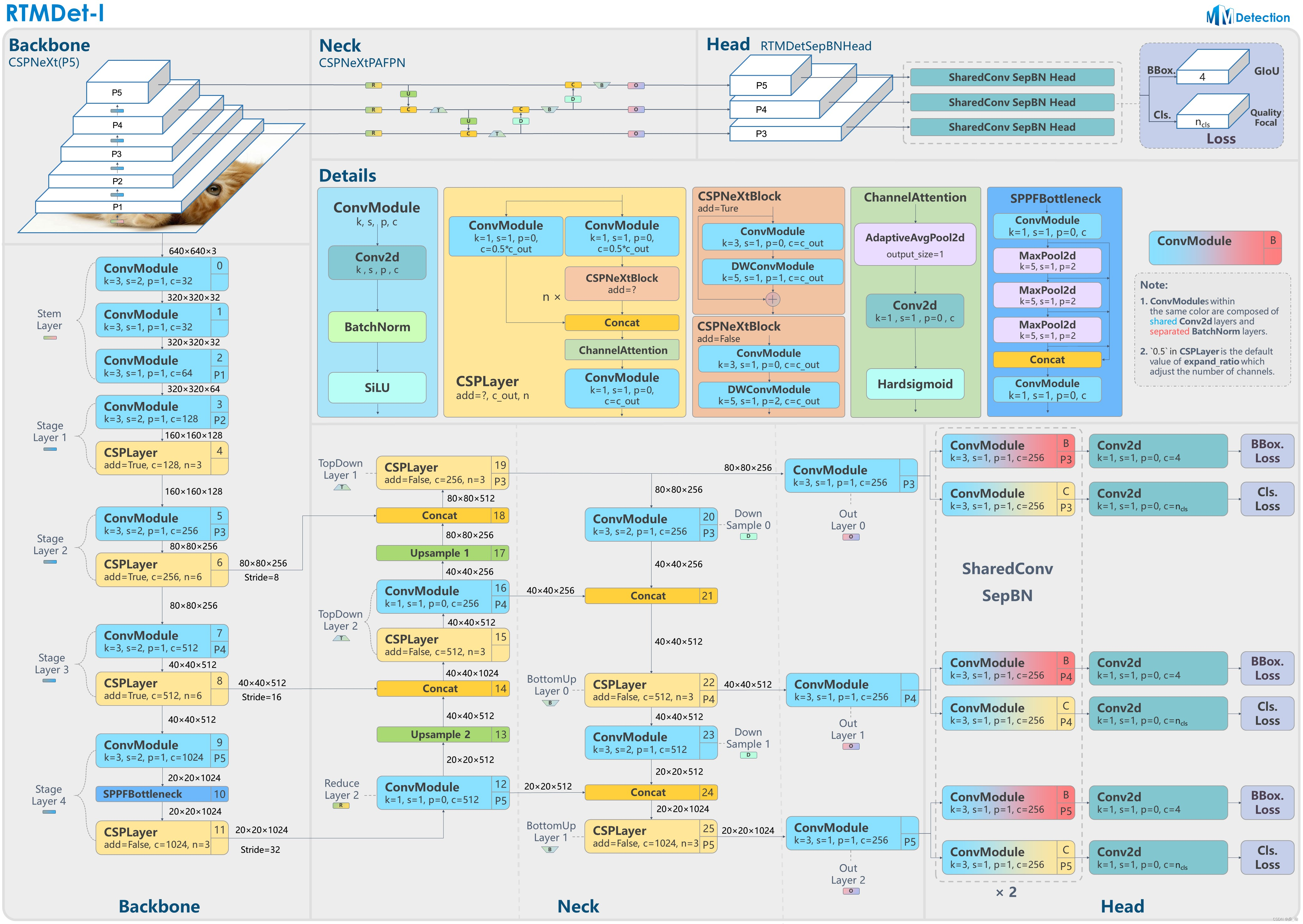
其模型架构图如上所示。RTMDet 是一个高性能低延时的检测算法,目前已经实现了目标检测、实例分割和旋转框检测任务。其简要描述为:为了获得更高效的模型架构,MMDetection 探索了一种具有骨干和 Neck 兼容容量的架构,由一个基本的构建块构成,其中包含大核深度卷积。MMDetection 进一步在动态标签分配中计算匹配成本时引入软标签,以提高准确性。结合更好的训练技巧,得到的目标检测器名为 RTMDet,在 NVIDIA 3090 GPU 上以超过 300 FPS 的速度实现了 52.8% 的 COCO AP,优于当前主流的工业检测器。RTMDet 在小/中/大/特大型模型尺寸中实现了最佳的参数-准确度权衡,适用于各种应用场景,并在实时实例分割和旋转对象检测方面取得了新的最先进性能。
cat 是一个单类的数据集,而 MMDetection 中提供的是 COCO 80 类配置,因此我们需要对一些重要参数通过配置来修改。
需要注意几个问题:
- 自定义数据集中最重要的是 metainfo 字段,用户在配置完成后要记得将其传给 dataset,否则不生效(有些用户在自定义数据集时候喜欢去 直接修改 coco.py 源码,这个是强烈不推荐的做法,正确做法是配置 metainfo 并传给 dataset)
- 如果用户 metainfo 配置不正确,通常会出现几种情况:(1) 出现 num_classes 不匹配错误 (2) loss_bbox 始终为 0 (3) 出现训练后评估结果为空等典型情况
- MMDetection 提供的学习率大部分都是基于 8 卡,如果你的总 bs 不同,一定要记得缩放学习率,否则有些算法很容易出现 NAN,具体参考 https://mmdetection.readthedocs.io/zh_CN/latest/user_guides/train.html#id3
首先我们在cat_data文件夹下面创建需要编写的配置文件(我一般喜欢在这个地方)
配置文件写好后,我们可以用下面py代码检测一下:
from mmdet.registry import DATASETS, VISUALIZERS
from mmengine.config import Config
from mmengine.registry import init_default_scope
import matplotlib.pyplot as plt
import os.path as osp

cfg = Config.fromfile('/gemini/code/mmdetection/cat_dataset/config_coco.py')

init_default_scope(cfg.get('default_scope', 'mmdet'))

dataset = DATASETS.build(cfg.train_dataloader.dataset)
visualizer = VISUALIZERS.build(cfg.visualizer)
visualizer.dataset_meta = dataset.metainfo

plt.figure(figsize=(16, 5))

# 只可视化前 8 张图片
for i in range(8):
   item=dataset[i]

   img = item['inputs'].permute(1, 2, 0).numpy()
   data_sample = item['data_samples'].numpy()
   gt_instances = data_sample.gt_instances
   img_path = osp.basename(item['data_samples'].img_path)

   gt_bboxes = gt_instances.get('bboxes', None)
   gt_instances.bboxes = gt_bboxes.tensor
   data_sample.gt_instances = gt_instances

   visualizer.add_datasample(
            osp.basename(img_path),
            img,
            data_sample,
            draw_pred=False,
            show=False)
   drawed_image=visualizer.get_image()

   plt.subplot(2, 4, i+1)
   plt.imshow(drawed_image[..., [2, 1, 0]])
   plt.title(f"{

      osp.basename(img_path)}")
   plt.xticks([])
   plt.yticks([])
plt.tight_layout()

如果显示以上信息,配置文件是没有问题的。
下面就可以开始run了
python3 tools/train.py cat_dataset/config_coco.py
