一、简介
win10, notebook ,python 3.6
朴素贝叶斯算法是有监督的学习算法,解决的是分类问题,如客户是否流失、是否值得投资、信用等级评定等多分类问题。
优点: 简单易懂、学习效率高、在某些领域的分类问题中能够与决策树、神经网络相媲美。
但由于该算法以自变量之间的独立(条件特征独立)性和连续变量的正态性假设为前提,就会导致算法精度在某种程度上受影响。
朴素贝叶斯推断的一些优点:
生成式模型,通过计算概率来进行分类,可以用来处理多分类问题。
对小规模的数据表现很好,适合多分类任务,适合增量式训练,算法也比较简单。
朴素贝叶斯推断的一些缺点:
对输入数据的表达形式很敏感。
由于朴素贝叶斯的“朴素”特点,所以会带来一些准确率上的损失。
需要计算先验概率,分类决策存在错误率。
参考:https://blog.csdn.net/c406495762/article/details/77341116
二、 原理
贝叶斯决策理论----条件概率----贝叶斯推断----例1----例2(朴素贝叶斯)
1、贝叶斯决策理论
朴素贝叶斯是贝叶斯决策理论的一部分,所以在讲述朴素贝叶斯之前有必要快速了解一下贝叶斯决策理论。
两类数据:

p1(x,y)表示数据点(x,y)属于类别1(图中红色圆点表示的类别)的概率,
p2(x,y)表示数据点(x,y)属于类别2(图中蓝色三角形表示的类别)的概率
- 如果p1(x,y) > p2(x,y),那么类别为1
- 如果p1(x,y) < p2(x,y),那么类别为2
即贝叶斯决策理论的核心思想:选择高概率对应的类别
2、条件概率与全概率
条件概率:在事件B发生的情况下,事件A发生的概率,用P(A|B)来表示
推导如图:

3、贝叶斯推断
- P(A)称为"先验概率"(Prior probability),即在B事件发生之前,我们对A事件概率的一个判断。
- P(A|B)称为"后验概率"(Posterior probability),即在B事件发生之后,我们对A事件概率的重新评估。
- P(B|A)/P(B)称为"可能性函数"(Likelyhood),这是一个调整因子,使得预估概率更接近真实概率。
可以理解为:
后验概率 = 先验概率 x 调整因子
即贝叶斯推断:我们先预估一个"先验概率",然后加入实验结果,看这个实验到底是增强还是削弱了"先验概率",由此得到更接近事实的"后验概率"。
- "可能性函数"P(B|A)/P(B)>1:意味着"先验概率"被增强,事件A的发生的可能性变大;
- "可能性函数"=1: 意味着B事件无助于判断事件A的可能性;
- "可能性函数"<1: 意味着"先验概率"被削弱,事件A的可能性变小。
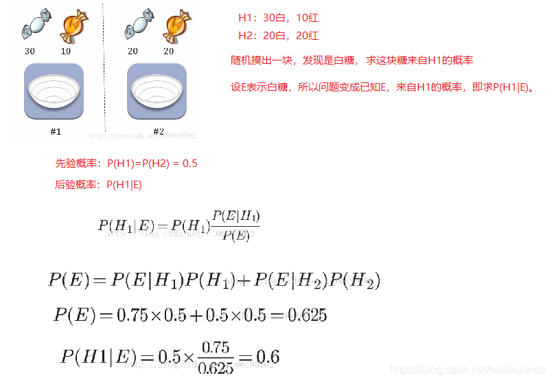
4、举例1
先验概率:
由于这两个碗是一样的,所以P(H1)=P(H2),也就是说,在取出白糖之前,这两个碗被选中的概率相同。
因此,P(H1)=0.5,我们把这个概率就叫做"先验概率",即没有做实验之前,来自一号碗的概率是0.5。
后验概率:
E表示白糖,所以问题就变成了在已知E的情况下,来自一号碗的概率有多大,即求P(H1|E)。
我们把这个概率叫做"后验概率",即在E事件发生之后,对P(H1)的修正。
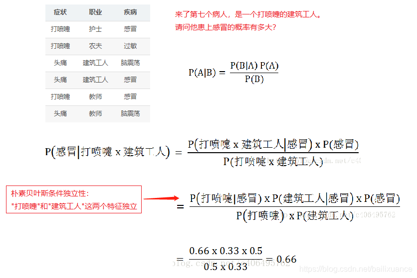
5、举例2
贝叶斯和朴素贝叶斯的概念是不同的,区别就在于“朴素”二字,朴素贝叶斯对条件个概率分布做了条件独立性的假设。
贝叶斯分类器的基本方法:在统计资料的基础上,依据某些特征,计算各个类别的概率,从而实现分类。
三、代码实现侮辱性言论过滤
1、整体过程:
文本切分----》向量化----》计算词频----》计算后验概率预测
如下图:
2、生成文本词典,并对文本进行向量化:
import numpy as np

# 切分的词条
postingList=[['my', 'dog', 'has', 'flea', 'problems', 'help', 'please'],
            ['maybe', 'not', 'take', 'him', 'to', 'dog', 'park', 'stupid'],
            ['my', 'dalmation', 'is', 'so', 'cute', 'I', 'love', 'him'],
            ['stop', 'posting', 'stupid', 'worthless', 'garbage'],
            ['mr', 'licks', 'ate', 'my', 'steak', 'how', 'to', 'stop', 'him'],
            ['quit', 'buying', 'worthless', 'dog', 'food', 'stupid']]
# 标签
classVec = [0,1,0,1,0,1]

# 转换为词条向量
def setOfWords2Vec(vocabList, inputSet):
    returnVec = [0] * len(vocabList)                                    #创建一个其中所含元素都为0的向量
    for word in inputSet:                                                #遍历每个词条
        if word in vocabList:                                            #如果词条存在于词汇表中,则置1
            returnVec[vocabList.index(word)] = 1
        else: print("the word: %s is not in my Vocabulary!" % word)
    return returnVec

# 单词词典,是一个集合
def createVocabList(dataSet):
    vocabSet = set([])                      #创建一个空的不重复列表
    for document in dataSet:
        vocabSet = vocabSet | set(document) #取并集
    return list(vocabSet)

myVocabList = createVocabList(postingList)
print('myVocabList:\n',myVocabList)

trainMat = []
for postinDoc in postingList:
    trainMat.append(setOfWords2Vec(myVocabList, postinDoc))
print('trainMat:\n', trainMat)
结果如下:
myVocabList:
 ['take', 'him', 'stupid', 'problems', 'help', 'mr', 'please', 'not', 'dalmation', 'my', 'has', 'buying', 'worthless', 'licks', 'to', 'is', 'love', 'quit', 'food', 'park', 'so', 'ate', 'dog', 'steak', 'I', 'cute', 'garbage', 'posting', 'how', 'stop', 'flea', 'maybe']
trainMat:
 [[0, 0, 0, 1, 1, 0, 1, 0, 0, 1, 1, 0, 0, 0, 0, 0, 0, 0, 0, 0, 0, 0, 1, 0, 0, 0, 0, 0, 0, 0, 1, 0], [1, 1, 1, 0, 0, 0, 0, 1, 0, 0, 0, 0, 0, 0, 1, 0, 0, 0, 0, 1, 0, 0, 1, 0, 0, 0, 0, 0, 0, 0, 0, 1], [0, 1, 0, 0, 0, 0, 0, 0, 1, 1, 0, 0, 0, 0, 0, 1, 1, 0, 0, 0, 1, 0, 0, 0, 1, 1, 0, 0, 0, 0, 0, 0], [0, 0, 1, 0, 0, 0, 0, 0, 0, 0, 0, 0, 1, 0, 0, 0, 0, 0, 0, 0, 0, 0, 0, 0, 0, 0, 1, 1, 0, 1, 0, 0], [0, 1, 0, 0, 0, 1, 0, 0, 0, 1, 0, 0, 0, 1, 1, 0, 0, 0, 0, 0, 0, 1, 0, 1, 0, 0, 0, 0, 1, 1, 0, 0], [0, 0, 1, 0, 0, 0, 0, 0, 0, 0, 0, 1, 1, 0, 0, 0, 0, 1, 1, 0, 0, 0, 1, 0, 0, 0, 0, 0, 0, 0, 0, 0]]
3、训练,即求训练样本中:
- p0V:在非侮辱类中,每个单词出现的频率
- p1V:在非侮辱类中,每个单词出现的频率
- pAb:侮辱类样本占的比率
def trainNB0(trainMatrix,trainCategory):
    numTrainDocs = len(trainMatrix)                            #计算训练的文档数目
    numWords = len(trainMatrix[0])                            #计算每篇文档的词条数
    pAbusive = sum(trainCategory)/float(numTrainDocs)        #文档属于侮辱类的概率

    '''
    未进行拉普拉斯平滑
    p0Num = np.zeros(numWords);
    p1Num = np.zeros(numWords)
    p0Denom = 0.0;
    p1Denom = 0.0
    '''
    # 创建numpy.ones数组,词条出现数初始化为2,拉普拉斯平滑
    p0Num = np.ones(numWords)
    p1Num = np.ones(numWords)
    # 分母初始化为2,拉普拉斯平滑
    p0Denom = 2.0
    p1Denom = 2.0
    for i in range(numTrainDocs):
        if trainCategory[i] == 1:                            #统计属于侮辱类的条件概率所需的数据,即P(w0|1),P(w1|1),P(w2|1)···
            p1Num += trainMatrix[i]
            p1Denom += sum(trainMatrix[i])
        else:                                                #统计属于非侮辱类的条件概率所需的数据,即P(w0|0),P(w1|0),P(w2|0)···
            p0Num += trainMatrix[i]
            p0Denom += sum(trainMatrix[i])
    p1Vect = np.log(p1Num/p1Denom)                            #取对数,防止下溢出
    p0Vect = np.log(p0Num/p0Denom)
    return p0Vect,p1Vect,pAbusive                            #返回属于侮辱类的条件概率数组,属于非侮辱类的条件概率数组,文档属于侮辱类的概率

p0V, p1V, pAb = trainNB0(trainMat, classVec)
4、预测:
def classifyNB(vec2Classify, p0Vec, p1Vec, pClass1):
    p1 = sum(vec2Classify * p1Vec) + np.log(pClass1)        #对应元素相乘。logA * B = logA + logB,所以这里加上log(pClass1)
    p0 = sum(vec2Classify * p0Vec) + np.log(1.0 - pClass1)
    if p1 > p0:
        return 1
    else:
        return 0


def testingNB():
    testEntry = ['love', 'my', 'dalmation']
    # 文本向量化
    thisDoc = np.array(setOfWords2Vec(myVocabList, testEntry))
    if classifyNB(thisDoc,p0V,p1V,pAb):
        print(testEntry,'属于侮辱类')
    else:
        print(testEntry,'属于非侮辱类')


    testEntry = ['stupid', 'garbage']
    thisDoc = np.array(setOfWords2Vec(myVocabList, testEntry))
    if classifyNB(thisDoc,p0V,p1V,pAb):
        print(testEntry,'属于侮辱类')
    else:
        print(testEntry,'属于非侮辱类')

testingNB()
结果:
['love', 'my', 'dalmation'] 属于非侮辱类
['stupid', 'garbage'] 属于侮辱类
四、代码实现垃圾邮件过滤
1、流程:
文本----向量化----训练----预测
样本:25个垃圾邮件,25个非垃圾邮件,
import re
import numpy as np
import random

# 分词
def textParse(bigString):                                                   #将字符串转换为字符列表
    listOfTokens = re.split(r'\W*', bigString)                              #将特殊符号作为切分标志进行字符串切分,即非字母、非数字
    return [tok.lower() for tok in listOfTokens if len(tok) > 2]            #除了单个字母,例如大写的I,其它单词变成小写

# 创建词典
def createVocabList(dataSet):
    vocabSet = set([])                      #创建一个空的不重复列表
    for document in dataSet:
        vocabSet = vocabSet | set(document) #取并集
    return list(vocabSet)

# 向量化
def setOfWords2Vec(vocabList, inputSet):
    returnVec = [0] * len(vocabList)                                    #创建一个其中所含元素都为0的向量
    for word in inputSet:                                                #遍历每个词条
        if word in vocabList:                                            #如果词条存在于词汇表中,则置1
            returnVec[vocabList.index(word)] = 1
        else: print("the word: %s is not in my Vocabulary!" % word)
    return returnVec                                                    #返回文档向量

# 样本字典
def bagOfWords2VecMN(vocabList, inputSet):
    returnVec = [0]*len(vocabList)                                        #创建一个其中所含元素都为0的向量
    for word in inputSet:                                                #遍历每个词条
        if word in vocabList:                                            #如果词条存在于词汇表中,则计数加一
            returnVec[vocabList.index(word)] += 1
    return returnVec                                                    #返回词袋模型
训练:
def trainNB0(trainMatrix,trainCategory):
    numTrainDocs = len(trainMatrix)                            #计算训练的文档数目
    numWords = len(trainMatrix[0])                            #计算每篇文档的词条数
    pAbusive = sum(trainCategory)/float(numTrainDocs)        #文档属于侮辱类的概率
    p0Num = np.ones(numWords); p1Num = np.ones(numWords)    #创建numpy.ones数组,词条出现数初始化为1,拉普拉斯平滑
    p0Denom = 2.0; p1Denom = 2.0                            #分母初始化为2,拉普拉斯平滑
    for i in range(numTrainDocs):
        if trainCategory[i] == 1:                            #统计属于侮辱类的条件概率所需的数据,即P(w0|1),P(w1|1),P(w2|1)···
            p1Num += trainMatrix[i]
            p1Denom += sum(trainMatrix[i])
        else:                                                #统计属于非侮辱类的条件概率所需的数据,即P(w0|0),P(w1|0),P(w2|0)···
            p0Num += trainMatrix[i]
            p0Denom += sum(trainMatrix[i])
    p1Vect = np.log(p1Num/p1Denom)                            #取对数,防止下溢出
    p0Vect = np.log(p0Num/p0Denom)
    return p0Vect,p1Vect,pAbusive                            #返回属于侮辱类的条件概率数组,属于非侮辱类的条件概率数组,文档属于侮辱类的概率
预测
def classifyNB(vec2Classify, p0Vec, p1Vec, pClass1):
    p1 = sum(vec2Classify * p1Vec) + np.log(pClass1)        #对应元素相乘。logA * B = logA + logB,所以这里加上log(pClass1)
    p0 = sum(vec2Classify * p0Vec) + np.log(1.0 - pClass1)
    if p1 > p0:
        return 1
    else:
        return 0
def spamTest():
    docList = []; classList = []; fullText = []
    for i in range(1, 26):                                                  #遍历25个txt文件
        # 垃圾邮件
        wordList = textParse(open('email/spam/%d.txt' % i, 'r').read())     #读取每个垃圾邮件,并字符串转换成字符串列表
        docList.append(wordList)
        fullText.append(wordList)
        classList.append(1)                                                 #标记垃圾邮件,1表示垃圾文件

        # 非垃圾邮件
        wordList = textParse(open('email/ham/%d.txt' % i, 'r').read())      #读取每个非垃圾邮件,并字符串转换成字符串列表
        docList.append(wordList)
        fullText.append(wordList)
        classList.append(0)                                                 #标记非垃圾邮件,1表示垃圾文件
    # 词汇表
    vocabList = createVocabList(docList)                                    #创建词汇表,不重复
    # print(vocabList)

    # 数据集切分
    trainingSet = list(range(50)); testSet = []                             #创建存储训练集的索引值的列表和测试集的索引值的列表
    for i in range(10):                                                     #从50个邮件中,随机挑选出40个作为训练集,10个做测试集
        randIndex = int(random.uniform(0, len(trainingSet)))                #随机选取索索引值
        testSet.append(trainingSet[randIndex])                              #添加测试集的索引值
        del(trainingSet[randIndex])                                         #在训练集列表中删除添加到测试集的索引值
    trainMat = []; trainClasses = []                                        #创建训练集矩阵和训练集类别标签系向量
    for docIndex in trainingSet:                                            #遍历训练集
        trainMat.append(setOfWords2Vec(vocabList, docList[docIndex]))       #将生成的词集模型添加到训练矩阵中
        trainClasses.append(classList[docIndex])                            #将类别添加到训练集类别标签系向量中
    p0V, p1V, pSpam = trainNB0(np.array(trainMat), np.array(trainClasses))  #训练朴素贝叶斯模型
    errorCount = 0                                                          #错误分类计数
    for docIndex in testSet:                                                #遍历测试集
        wordVector = setOfWords2Vec(vocabList, docList[docIndex])           #测试集的词集模型
        if classifyNB(np.array(wordVector), p0V, p1V, pSpam) != classList[docIndex]:    #如果分类错误
            errorCount += 1                                                 #错误计数加1
            print("分类错误的测试集:",docList[docIndex])
    print('错误率:%.2f%%' % (float(errorCount) / len(testSet) * 100))


spamTest()
结果:
分类错误的测试集: ['scifinance', 'now', 'automatically', 'generates', 'gpu', 'enabled', 'pricing', 'risk', 'model', 'source', 'code', 'that', 'runs', '300x', 'faster', 'than', 'serial', 'code', 'using', 'new', 'nvidia', 'fermi', 'class', 'tesla', 'series', 'gpu', 'scifinance', 'derivatives', 'pricing', 'and', 'risk', 'model', 'development', 'tool', 'that', 'automatically', 'generates', 'and', 'gpu', 'enabled', 'source', 'code', 'from', 'concise', 'high', 'level', 'model', 'specifications', 'parallel', 'computing', 'cuda', 'programming', 'expertise', 'required', 'scifinance', 'automatic', 'gpu', 'enabled', 'monte', 'carlo', 'pricing', 'model', 'source', 'code', 'generation', 'capabilities', 'have', 'been', 'significantly', 'extended', 'the', 'latest', 'release', 'this', 'includes']
错误率:10.00%
可见:大部分精力都花在了数据处理上面了。
训练算法使用之前建立的trainNB0()函数。
五、基于SKLearn朴素贝叶斯之新浪新闻分类
1、scikit-learn朴素贝叶斯简介
在scikit-learn中,一共有3个朴素贝叶斯的分类算法类。分别是GaussianNB,MultinomialNB和BernoulliNB。
- GaussianNB:先验为高斯分布的朴素贝叶斯
- MultinomialNB:先验为多项式分布的朴素贝叶斯
- BernoulliNB:先验为伯努利分布的朴素贝叶斯
对于新闻分类,属于多分类问题。我们可以使用MultinamialNB()完成我们的新闻分类问题。
MultinomialNB假设特征的先验概率为多项式分布,即如下式:
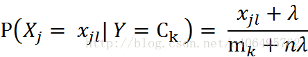
其中,P(Xj = Xjl | Y = Ck)是第k个类别的第j维特征的第l个取值条件概率。mk是训练集中输出为第k类的样本个数。λ为一个大于0的常数,尝尝取值为1,即拉普拉斯平滑,也可以取其他值。
2、MultinamialNB参数:
下MultinamialNB这个函数,只有3个参数:

- alpha:浮点型可选参数,默认为1.0,其实就是添加拉普拉斯平滑,即为上述公式中的λ ,如果这个参数设置为0,就是不添加平滑;
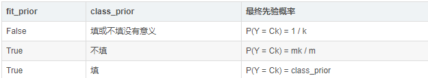
- fit_prior:布尔型可选参数,默认为True。布尔参数fit_prior表示是否要考虑先验概率,如果是false,则所有的样本类别输出都有相同的类别先验概率。否则可以自己用第三个参数class_prior输入先验概率,或者不输入第三个参数class_prior让MultinomialNB自己从训练集样本来计算先验概率,此时的先验概率为P(Y=Ck)=mk/m。其中m为训练集样本总数量,mk为输出为第k类别的训练集样本数。
- class_prior:可选参数,默认为None。
3、代码
流程:文本分词----特征选择(去停用词等)----去高频词----训练分类----预测
数据处理,切分成训练集,测试集
from sklearn.naive_bayes import MultinomialNB
import matplotlib.pyplot as plt
import os
import random
import jieba

# 数据预处理,把原始数据(txt文件)整理成测试集,训练集,词典
def TextProcessing(folder_path, test_size = 0.2):
    folder_list = os.listdir(folder_path)                        #查看folder_path下的文件
    data_list = []                                                #数据集数据
    class_list = []                                                #数据集类别

    #遍历每个子文件夹
    for folder in folder_list:
        new_folder_path = os.path.join(folder_path, folder)        #根据子文件夹,生成新的路径
        files = os.listdir(new_folder_path)                        #存放子文件夹下的txt文件的列表

        j = 1
        #遍历每个txt文件
        for file in files:
            if j > 100:                                            #每类txt样本数最多100个
                break
            with open(os.path.join(new_folder_path, file), 'r', encoding = 'utf-8') as f:    #打开txt文件
                raw = f.read()

            word_cut = jieba.cut(raw, cut_all = False)            #精简模式,返回一个可迭代的generator
            word_list = list(word_cut)                            #generator转换为list

            data_list.append(word_list)                            #添加数据集数据
            class_list.append(folder)                            #添加数据集类别
            j += 1

    data_class_list = list(zip(data_list, class_list))            #zip压缩合并,将数据与标签对应压缩
    random.shuffle(data_class_list)                                #将data_class_list乱序
    index = int(len(data_class_list) * test_size) + 1            #训练集和测试集切分的索引值
    train_list = data_class_list[index:]                        #训练集
    test_list = data_class_list[:index]                            #测试集
    train_data_list, train_class_list = zip(*train_list)        #训练集解压缩
    test_data_list, test_class_list = zip(*test_list)            #测试集解压缩

    all_words_dict = {}                                            #统计训练集词频
    for word_list in train_data_list:
        for word in word_list:
            if word in all_words_dict.keys():
                all_words_dict[word] += 1
            else:
                all_words_dict[word] = 1

    #根据键的值倒序排序
    all_words_tuple_list = sorted(all_words_dict.items(), key = lambda f:f[1], reverse = True)
    all_words_list, all_words_nums = zip(*all_words_tuple_list)    #解压缩
    all_words_list = list(all_words_list)                        #转换成列表
    return all_words_list, train_data_list, test_data_list, train_class_list, test_class_list
停用词,去除高频词
# 停用词词典
def MakeWordsSet(words_file):
    words_set = set()                                            #创建set集合
    with open(words_file, 'r', encoding = 'utf-8') as f:        #打开文件
        for line in f.readlines():                                #一行一行读取
            word = line.strip()                                    #去回车
            if len(word) > 0:                                    #有文本,则添加到words_set中
                words_set.add(word)
    return words_set                                             #返回处理结果

# 去除高频词后的特征词词典
def words_dict(all_words_list, deleteN, stopwords_set = set()):
    feature_words = []
    n = 1
    for t in range(deleteN, len(all_words_list), 1):
        if n > 1000:                            #feature_words的维度为1000
            break
        #如果这个词不是数字,不是停用词,并且单词长度大于1小于5,那么这个词就可以作为特征词
        if not all_words_list[t].isdigit() and all_words_list[t] not in stopwords_set and 1 < len(all_words_list[t]) < 5:
            feature_words.append(all_words_list[t])
        n += 1
    return feature_words
向量化
# 将训练集和测试集向量化
def TextFeatures(train_data_list, test_data_list, feature_words):
    def text_features(text, feature_words):                        #出现在特征集中,则置1
        text_words = set(text)
        features = [1 if word in text_words else 0 for word in feature_words]
        return features
    train_feature_list = [text_features(text, feature_words) for text in train_data_list]
    test_feature_list = [text_features(text, feature_words) for text in test_data_list]
    return train_feature_list, test_feature_list                #返回结果
预测
# 使用SKLearn 中的贝叶斯函数进行预测
def TextClassifier(train_feature_list, test_feature_list, train_class_list, test_class_list):
    classifier = MultinomialNB().fit(train_feature_list, train_class_list)
    test_accuracy = classifier.score(test_feature_list, test_class_list)
    return test_accuracy
if __name__ == '__main__':
    folder_path = './SogouC/Sample'
    # 数据集划分
    all_words_list, train_data_list, test_data_list, train_class_list, test_class_list = TextProcessing(folder_path, test_size=0.2)

    # 停用词词典
    stopwords_file = './stopwords_cn.txt'
    stopwords_set = MakeWordsSet(stopwords_file)


    test_accuracy_list = []
    deleteNs = range(0, 1000, 20)                #0 20 40 60 ... 980
    for deleteN in deleteNs:
        # 去除高频词后的特征词词典
        feature_words = words_dict(all_words_list, deleteN, stopwords_set)
        # 将数据集向量化
        train_feature_list, test_feature_list = TextFeatures(train_data_list, test_data_list, feature_words)
        #预测
        test_accuracy = TextClassifier(train_feature_list, test_feature_list, train_class_list, test_class_list)
        test_accuracy_list.append(test_accuracy)

    plt.figure()
    plt.plot(deleteNs, test_accuracy_list)
    plt.title('Relationship of deleteNs and test_accuracy')
    plt.xlabel('deleteNs')
    plt.ylabel('test_accuracy')
    plt.show()
结果:

大部分精力同样是数据处理,
调用SKLearn中的函数十分简单