一. 逻辑回归
1.背景:使用逻辑回归预测学生是否会被大学录取。
数据集:
34.62365962451697,78.0246928153624,0
30.28671076822607,43.89499752400101,0
35.84740876993872,72.90219802708364,0
60.18259938620976,86.30855209546826,1
79.0327360507101,75.3443764369103,1
45.08327747668339,56.3163717815305,0
61.10666453684766,96.51142588489624,1
75.02474556738889,46.55401354116538,1
76.09878670226257,87.42056971926803,1
84.43281996120035,43.53339331072109,1
95.86155507093572,38.22527805795094,0
75.01365838958247,30.60326323428011,0
82.30705337399482,76.48196330235604,1
69.36458875970939,97.71869196188608,1
39.53833914367223,76.03681085115882,0
53.9710521485623,89.20735013750205,1
2.首先对数据进行可视化,代码如下:
主程序中绘图代码:
%% Initialization
clear ; close all; clc

%% Load Data
%  The first two columns contains the exam scores and the third column
%  contains the label.

data = load('ex2data1.txt');
X = data(:, [1, 2]); y = data(:, 3);

%% ==================== Part 1: Plotting ====================
%  We start the exercise by first plotting the data to understand the
%  the problem we are working with.

fprintf(['Plotting data with + indicating (y = 1) examples and o ' ...
         'indicating (y = 0) examples.\n']);

plotData(X, y);

% Put some labels
hold on;
% Labels and Legend
xlabel('Exam 1 score')
ylabel('Exam 2 score')

% Specified in plot order
legend('Admitted', 'Not admitted')
hold off;

fprintf('\nProgram paused. Press enter to continue.\n');
pause;
子函数plotData函数代码:
这里学习find函数的用法,它返回所有满足条件的元素的index
对于单行或者单列的矩阵find()直接返回对应的index组成的单行或单列的矩阵
对于多行多列矩阵[x,y]=find(),可以分别获得行号列号
function plotData(X, y)
%PLOTDATA Plots the data points X and y into a new figure
%   PLOTDATA(x,y) plots the data points with + for the positive examples
%   and o for the negative examples. X is assumed to be a Mx2 matrix.

% Create New Figure
figure; hold on;

% ====================== YOUR CODE HERE ======================
% Instructions: Plot the positive and negative examples on a
%               2D plot, using the option 'k+' for the positive
%               examples and 'ko' for the negative examples.
%% 绘图
pos = find(y==1); %找到通过学生的序号向量
neg = find(y==0); %找到未通过学生的序号向量
%画出来是黑色十字架
plot(X(pos,1),X(pos,2),'k+','LineWidth',2,'MarkerSize',7); %使用+绘制 通过的学生
hold on;
%画出来黄色的圆圈
plot(X(neg,1),X(neg,2),'ko','MarkerFaceColor','y','MarkerSize',7); %使用o绘制 未通过的学生
% =========================================================================

hold off;

end

Logistic函数
对于任意的x值,对应的y值都在区间(0,1)内。
函数公式为: ,
,
扫描二维码关注公众号,回复:
2476254 查看本文章

这个函数的曲线如下所示:
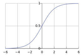
很像一个“S”型吧,所以又叫 sigmoid曲线(S型曲线)。
sigmoid函数的实现,代码如下: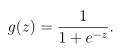
function g = sigmoid(z)
%SIGMOID Compute sigmoid function
%   g = SIGMOID(z) computes the sigmoid of z.

% You need to return the following variables correctly
g = zeros(size(z));

% ====================== YOUR CODE HERE ======================
% Instructions: Compute the sigmoid of each value of z (z can be a matrix,
%               vector or scalar).
g = zeros(size(z));%初始化g
temp=-z;
temp=e.^temp;
temp=temp+1;
temp=1./temp;
g=temp;
% =============================================================
end
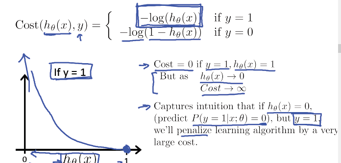
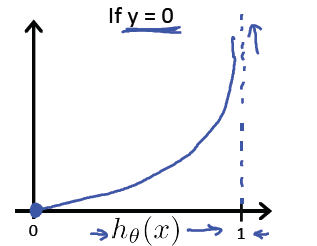
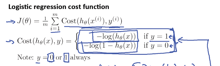
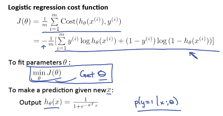
逻辑回归的代价函数:
逻辑回归的代价函数很可能是一个非凸函数(non-convex),有很多局部最优点,所以如果用梯度下降法,不能保证会收敛到全局最小值。
逻辑回归的代价函数代码如下:


Cost Function & Gradient
function [J, grad] = costFunction(theta, X, y)
%COSTFUNCTION Compute cost and gradient for logistic regression
% J = COSTFUNCTION(theta, X, y) computes the cost of using theta as the
% parameter for logistic regression and the gradient of the cost
% w.r.t. to the parameters.
% Initialize some useful values
m = length(y); % number of training examples
% You need to return the following variables correctly
J = 0;
grad = zeros(size(theta));
% ====================== YOUR CODE HERE ======================
% Instructions: Compute the cost of a particular choice of theta.
% You should set J to the cost.
% Compute the partial derivatives and set grad to the partial
% derivatives of the cost w.r.t. each parameter in theta
%
% Note: grad should have the same dimensions as theta
%
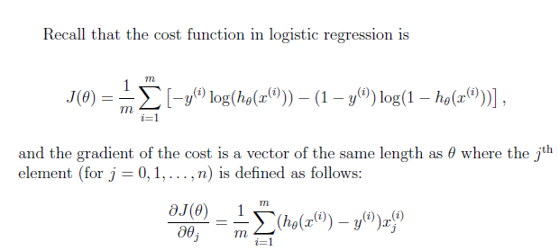
J = 1/m*(-(y')*log(sigmoid(X*theta))-(1-y)'*log(1-sigmoid(X*theta))); %计算代价函数
grad = zeros(size(theta));
grad = 1/m*X'*(sigmoid(X*theta)-y); %求梯度
% =============================================================
end
%% ============ Part 2: Compute Cost and Gradient ============
%  In this part of the exercise, you will implement the cost and gradient
%  for logistic regression. You neeed to complete the code in
%  costFunction.m

%  Setup the data matrix appropriately, and add ones for the intercept term
[m, n] = size(X);

% Add intercept term to x and X_test
X = [ones(m, 1) X];

% Initialize fitting parameters
initial_theta = zeros(n + 1, 1);

% Compute and display initial cost and gradient
[cost, grad] = costFunction(initial_theta, X, y);

fprintf('Cost at initial theta (zeros): %f\n', cost);
fprintf('Expected cost (approx): 0.693\n');
fprintf('Gradient at initial theta (zeros): \n');
fprintf(' %f \n', grad);
fprintf('Expected gradients (approx):\n -0.1000\n -12.0092\n -11.2628\n');

% Compute and display cost and gradient with non-zero theta
test_theta = [-24; 0.2; 0.2];
[cost, grad] = costFunction(test_theta, X, y);

fprintf('\nCost at test theta: %f\n', cost);
fprintf('Expected cost (approx): 0.218\n');
fprintf('Gradient at test theta: \n');
fprintf(' %f \n', grad);
fprintf('Expected gradients (approx):\n 0.043\n 2.566\n 2.647\n');

fprintf('\nProgram paused. Press enter to continue.\n');
pause;
%% ============= Part 3: Optimizing using fminunc  =============
%代替梯度下降的优化方法fminunc()
%  In this exercise, you will use a built-in function (fminunc) to find the
%  optimal parameters theta.

%  Set options for fminunc
options = optimset('GradObj', 'on', 'MaxIter', 400);

%  Run fminunc to obtain the optimal theta
%  This function will return theta and the cost
[theta, cost] = ...
	fminunc(@(t)(costFunction(t, X, y)), initial_theta, options);

% Print theta to screen
fprintf('Cost at theta found by fminunc: %f\n', cost);
fprintf('Expected cost (approx): 0.203\n');
fprintf('theta: \n');
fprintf(' %f \n', theta);
fprintf('Expected theta (approx):\n');
fprintf(' -25.161\n 0.206\n 0.201\n');

% Plot Boundary
plotDecisionBoundary(theta, X, y);

% Put some labels
hold on;
% Labels and Legend
xlabel('Exam 1 score')
ylabel('Exam 2 score')

% Specified in plot order
legend('Admitted', 'Not admitted')
hold off;

fprintf('\nProgram paused. Press enter to continue.\n');
pause;
运行结果:

预测部分:

function p = predict(theta, X)
%PREDICT Predict whether the label is 0 or 1 using learned logistic
%regression parameters theta
% p = PREDICT(theta, X) computes the predictions for X using a
% threshold at 0.5 (i.e., if sigmoid(theta'*x) >= 0.5, predict 1)
m = size(X, 1); % Number of training examples
% You need to return the following variables correctly
p = zeros(m, 1);
% ====================== YOUR CODE HERE ======================
% Instructions: Complete the following code to make predictions using
% your learned logistic regression parameters.
% You should set p to a vector of 0's and 1's
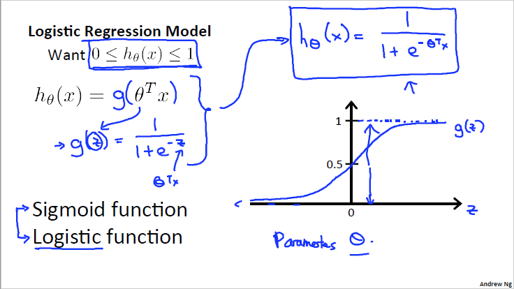
% 逻辑回归模型的假设是: hθ(x)=g(θTX)
% 将sigmoid函数代入逻辑回归模型假设
p_medium=sigmoid(X*theta);
% 在逻辑回归中,我们预测:
% 当hθ(x)大于等于0.5时,预测y=1
% 当hθ(x)小于0.5时,预测y=0
pos=find(p_medium >= 0.5);
p(pos,1)=1;
% =========================================================================
end
%% ============== Part 4: Predict and Accuracies ==============
%  预测给定数据,既分类
%  After learning the parameters, you'll like to use it to predict the outcomes
%  on unseen data. In this part, you will use the logistic regression model
%  to predict the probability that a student with score 45 on exam 1 and
%  score 85 on exam 2 will be admitted.
%  在学习参数之后,您将使用它来预测未见数据的结果。 在本部分中,您将使用逻辑回归模型
% 预测考试1中考试成绩为45考试2中的85分将被录取的学生的概率
%
%  Furthermore, you will compute the training and test set accuracies of
%  our model.
%
%  Your task is to complete the code in predict.m

%  Predict probability for a student with score 45 on exam 1
%  and score 85 on exam 2
% 针对一个输入特征 来看一个输入特征灌入逻辑回归模型 最终预测出来结果跟1实际差多少
prob = sigmoid([1 45 85] * theta);
fprintf(['For a student with scores 45 and 85, we predict an admission ' ...
         'probability of %f\n'], prob);
fprintf('Expected value: 0.775 +/- 0.002\n\n');

% Compute accuracy on our training set
% 得到所有训练数据 灌入逻辑回归模型中 最终预测出来值
p = predict(theta, X);
% 拿得到的实际预测值 跟实际值 看最终判断正确率
fprintf('Train Accuracy: %f\n', mean(double(p == y)) * 100);
fprintf('Expected accuracy (approx): 89.0\n');
fprintf('\n');
Regularized logistic regression
Visualization
这里使用的数据是一个工厂对生产的芯片进行的质量检查相关数据,包含2次不同测试的结果和是否合格产品的结果
0.051267,0.69956,1
-0.092742,0.68494,1
-0.21371,0.69225,1
-0.375,0.50219,1
-0.51325,0.46564,1
-0.52477,0.2098,1
-0.39804,0.034357,1
-0.30588,-0.19225,1
0.016705,-0.40424,1
0.13191,-0.51389,1
0.38537,-0.56506,1
0.52938,-0.5212,1
0.63882,-0.24342,1
0.73675,-0.18494,1
0.54666,0.48757,1
0.322,0.5826,1
0.16647,0.53874,1
-0.046659,0.81652,1
-0.17339,0.69956,1
-0.47869,0.63377,1
-0.60541,0.59722,1
-0.62846,0.33406,1
-0.59389,0.005117,1
-0.42108,-0.27266,1
-0.11578,-0.39693,1
0.20104,-0.60161,1
0.46601,-0.53582,1
0.67339,-0.53582,1
%% Machine Learning Online Class - Exercise 2: Logistic Regression
%
%  Instructions
%  ------------
%
%  This file contains code that helps you get started on the second part
%  of the exercise which covers regularization with logistic regression.
%
%  You will need to complete the following functions in this exericse:
%
%     sigmoid.m
%     costFunction.m
%     predict.m
%     costFunctionReg.m
%
%  For this exercise, you will not need to change any code in this file,
%  or any other files other than those mentioned above.
%

%% Initialization
clear ; close all; clc

%% Load Data
%  The first two columns contains the X values and the third column
%  contains the label (y).

data = load('ex2data2.txt');
X = data(:, [1, 2]); y = data(:, 3);

plotData(X, y);

% Put some labels
hold on;

% Labels and Legend
xlabel('Microchip Test 1')
ylabel('Microchip Test 2')

% Specified in plot order
legend('y = 1', 'y = 0')
hold off;
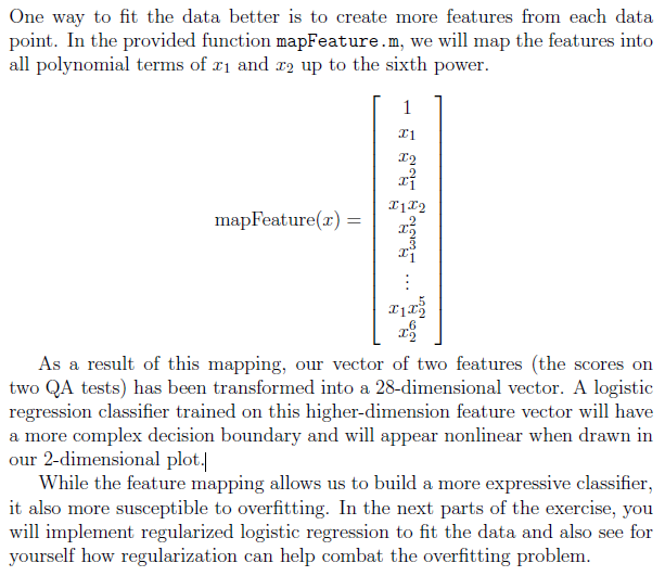
正则化的逻辑回归模型

%% =========== Part 1: Regularized Logistic Regression ============
%  In this part, you are given a dataset with data points that are not
%  linearly separable. However, you would still like to use logistic
%  regression to classify the data points.
%
%  To do so, you introduce more features to use -- in particular, you add
%  polynomial features to our data matrix (similar to polynomial
%  regression).
%

% Add Polynomial Features

% Note that mapFeature also adds a column of ones for us, so the intercept
% term is handled
X = mapFeature(X(:,1), X(:,2));

% Initialize fitting parameters
initial_theta = zeros(size(X, 2), 1);

% Set regularization parameter lambda to 1
% 正则化参数
lambda = 1;

% Compute and display initial cost and gradient for regularized logistic
% regression
[cost, grad] = costFunctionReg(initial_theta, X, y, lambda);

fprintf('Cost at initial theta (zeros): %f\n', cost);
fprintf('Expected cost (approx): 0.693\n');
fprintf('Gradient at initial theta (zeros) - first five values only:\n');
fprintf(' %f \n', grad(1:5));
fprintf('Expected gradients (approx) - first five values only:\n');
fprintf(' 0.0085\n 0.0188\n 0.0001\n 0.0503\n 0.0115\n');

fprintf('\nProgram paused. Press enter to continue.\n');
pause;

% Compute and display cost and gradient
% with all-ones theta and lambda = 10
test_theta = ones(size(X,2),1);
[cost, grad] = costFunctionReg(test_theta, X, y, 10);

fprintf('\nCost at test theta (with lambda = 10): %f\n', cost);
fprintf('Expected cost (approx): 3.16\n');
fprintf('Gradient at test theta - first five values only:\n');
fprintf(' %f \n', grad(1:5));
fprintf('Expected gradients (approx) - first five values only:\n');
fprintf(' 0.3460\n 0.1614\n 0.1948\n 0.2269\n 0.0922\n');

fprintf('\nProgram paused. Press enter to continue.\n');
pause;
function [J, grad] = costFunctionReg(theta, X, y, lambda)
%COSTFUNCTIONREG Compute cost and gradient for logistic regression with regularization
% J = COSTFUNCTIONREG(theta, X, y, lambda) computes the cost of using
% theta as the parameter for regularized logistic regression and the
% gradient of the cost w.r.t. to the parameters.
% Initialize some useful values
m = length(y); % number of training examples
% You need to return the following variables correctly
J = 0;
grad = zeros(size(theta));
% ====================== YOUR CODE HERE ======================
% Instructions: Compute the cost of a particular choice of theta.
% You should set J to the cost.
% Compute the partial derivatives and set grad to the partial
% derivatives of the cost w.r.t. each parameter in theta
h = sigmoid(X*theta);
t = theta(2:length(theta),1);
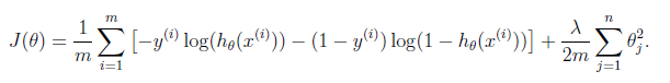
% 正则化线性回归的代价函数为:
J = m^-1 * sum(((-1) * y.*log(h))-((1- y).*log(1 - h))) + 0.5*(lambda/m) * sum(t.^2);
% 如果我们要使用梯度下降法令这个代价函数最小化 下面是拿到代价函数的求导 也就是梯度
grad = m^-1 * ((h-y)'*X)';
tmp = grad;
tmp = tmp + (lambda/m)*theta;
grad = [grad(1,1);tmp(2:length(theta),1)];
% =============================================================
end
Ploting the decision boundary
这里就使用的是上面函数的第二部分了。另外就是lamda取不同的值,可以从下面开得到对于fitting的影响
通过改变lamda(正则化参数)可以查看正则化参数影响下不同效果:

正则化和精度
%% ============= Part 2: Regularization and Accuracies =============
%  Optional Exercise:
%  In this part, you will get to try different values of lambda and
%  see how regularization affects the decision coundart
%
%  Try the following values of lambda (0, 1, 10, 100).
%
%  How does the decision boundary change when you vary lambda? How does
%  the training set accuracy vary?
%

% Initialize fitting parameters
initial_theta = zeros(size(X, 2), 1);

% Set regularization parameter lambda to 1 (you should vary this)
lambda = 1;

% Set Options
options = optimset('GradObj', 'on', 'MaxIter', 400);

% Optimize
[theta, J, exit_flag] = ...
	fminunc(@(t)(costFunctionReg(t, X, y, lambda)), initial_theta, options);

% Plot Boundary
plotDecisionBoundary(theta, X, y);
hold on;
title(sprintf('lambda = %g', lambda))

% Labels and Legend
xlabel('Microchip Test 1')
ylabel('Microchip Test 2')

legend('y = 1', 'y = 0', 'Decision boundary')
hold off;

% Compute accuracy on our training set
p = predict(theta, X);

fprintf('Train Accuracy: %f\n', mean(double(p == y)) * 100);
fprintf('Expected accuracy (with lambda = 1): 83.1 (approx)\n');

