exercise 7 —— K-means and PCA
在此下载Coursera-吴恩达-机器学习-全部编程练习答案
在本练习中,您将实现K均值聚类算法并将其应用于压缩图像。 在第二部分中,您将使用主成分分析来查找面部图像的低维表示。
1 K-means
先从二维的点开始,使用K-means进行分类。
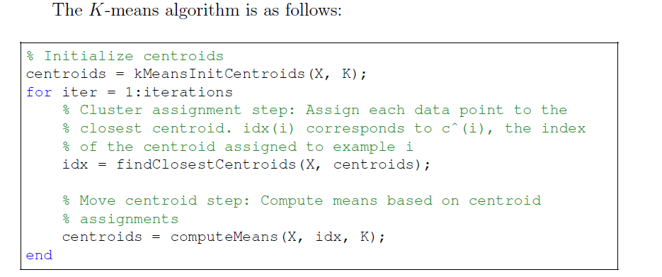
K-means步骤如上,在每次循环中,先对所有点更新分类,再更新每一类的中心坐标。
ex7.m中提供了一个例子,其中中 K 已经被手动初始化过了。
%% Machine Learning Online Class
%  Exercise 7 | Principle Component Analysis and K-Means Clustering
%
%  Instructions
%  ------------
%
%  This file contains code that helps you get started on the
%  exercise. You will need to complete the following functions:
%
%     pca.m
%     projectData.m
%     recoverData.m
%     computeCentroids.m
%     findClosestCentroids.m
%     kMeansInitCentroids.m
%
%  For this exercise, you will not need to change any code in this file,
%  or any other files other than those mentioned above.
%

%% Initialization
clear ; close all; clc

%% ================= Part 1: Find Closest Centroids ====================
%  To help you implement K-Means, we have divided the learning algorithm
%  into two functions -- findClosestCentroids and computeCentroids. In this
%  part, you should complete the code in the findClosestCentroids function.
%
fprintf('Finding closest centroids.\n\n');

% Load an example dataset that we will be using
load('ex7data2.mat');

% Select an initial set of centroids
K = 3; % 3 Centroids
initial_centroids = [3 3; 6 2; 8 5];

% Find the closest centroids for the examples using the
% initial_centroids
idx = findClosestCentroids(X, initial_centroids);

fprintf('Closest centroids for the first 3 examples: \n')
fprintf(' %d', idx(1:3));
fprintf('\n(the closest centroids should be 1, 3, 2 respectively)\n');

fprintf('Program paused. Press enter to continue.\n');
pause;
function idx = findClosestCentroids(X, centroids)
%FINDCLOSESTCENTROIDS computes the centroid memberships for every example
% idx = FINDCLOSESTCENTROIDS (X, centroids) returns the closest centroids
% in idx for a dataset X where each row is a single example. idx = m x 1
% vector of centroid assignments (i.e. each entry in range [1..K])
%
% Set K
K = size(centroids, 1);
% You need to return the following variables correctly.
idx = zeros(size(X,1), 1);
% ====================== YOUR CODE HERE ======================
% Instructions: Go over every example, find its closest centroid, and store
% the index inside idx at the appropriate location.
% Concretely, idx(i) should contain the index of the centroid
% closest to example i. Hence, it should be a value in the
% range 1..K
%
% Note: You can use a for-loop over the examples to compute this.
%
for i=1:size(X,1)
adj=sqrt((X(i,:)-centroids(1,:))*(X(i,:)-centroids(1,:))');
idx(i)=1;
for j=2:K
temp=sqrt((X(i,:)-centroids(j,:))*(X(i,:)-centroids(j,:))');
if(temp<adj)
idx(i)=j;
adj=temp;
end
end
end
% =============================================================
end
%% ===================== Part 2: Compute Means =========================
%  After implementing the closest centroids function, you should now
%  complete the computeCentroids function.
%
fprintf('\nComputing centroids means.\n\n');

%  Compute means based on the closest centroids found in the previous part.
centroids = computeCentroids(X, idx, K);

fprintf('Centroids computed after initial finding of closest centroids: \n')
fprintf(' %f %f \n' , centroids');
fprintf('\n(the centroids should be\n');
fprintf('   [ 2.428301 3.157924 ]\n');
fprintf('   [ 5.813503 2.633656 ]\n');
fprintf('   [ 7.119387 3.616684 ]\n\n');

fprintf('Program paused. Press enter to continue.\n');
pause;
function centroids = computeCentroids(X, idx, K)
%COMPUTECENTROIDS returns the new centroids by computing the means of the
%data points assigned to each centroid.
% centroids = COMPUTECENTROIDS(X, idx, K) returns the new centroids by
% computing the means of the data points assigned to each centroid. It is
% given a dataset X where each row is a single data point, a vector
% idx of centroid assignments (i.e. each entry in range [1..K]) for each
% example, and K, the number of centroids. You should return a matrix
% centroids, where each row of centroids is the mean of the data points
% assigned to it.
%
% Useful variables
[m n] = size(X);
% You need to return the following variables correctly.
centroids = zeros(K, n);
% ====================== YOUR CODE HERE ======================
% Instructions: Go over every centroid and compute mean of all points that
% belong to it. Concretely, the row vector centroids(i, :)
% should contain the mean of the data points assigned to
% centroid i.
%
% Note: You can use a for-loop over the centroids to compute this.
%
for i=1:K
if(size(find(idx==i),2)~=0)
centroids(i,:)=mean(X(find(idx==i),:));
else
centroids(i,:)=zeros(1,n);
end
end
% =============================================================
end
%% =================== Part 3: K-Means Clustering ======================
%  After you have completed the two functions computeCentroids and
%  findClosestCentroids, you have all the necessary pieces to run the
%  kMeans algorithm. In this part, you will run the K-Means algorithm on
%  the example dataset we have provided.
%
fprintf('\nRunning K-Means clustering on example dataset.\n\n');

% Load an example dataset
load('ex7data2.mat');

% Settings for running K-Means
K = 3;
max_iters = 10;

% For consistency, here we set centroids to specific values
% but in practice you want to generate them automatically, such as by
% settings them to be random examples (as can be seen in
% kMeansInitCentroids).
initial_centroids = [3 3; 6 2; 8 5];

% Run K-Means algorithm. The 'true' at the end tells our function to plot
% the progress of K-Means
[centroids, idx] = runkMeans(X, initial_centroids, max_iters, true);
fprintf('\nK-Means Done.\n\n');

fprintf('Program paused. Press enter to continue.\n');
pause;
我们要把点分成三类,迭代次数为10次。三类的中心点初始化为(3,3),(6,2),(8,5).
得到如下图像。(中间的图像略去,只展示开始和完成时的图像)
这是初始图像:
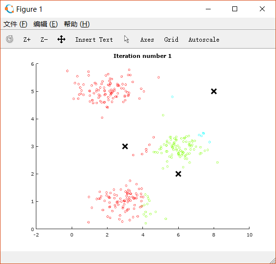


进行10次迭代后的图像:image
可以看到三堆点被很好地分成了三类。图片上同时也展示了中心点的移动轨迹。

%% ============= Part 4: K-Means Clustering on Pixels ===============
%  In this exercise, you will use K-Means to compress an image. To do this,
%  you will first run K-Means on the colors of the pixels in the image and
%  then you will map each pixel onto its closest centroid.
%
%  You should now complete the code in kMeansInitCentroids.m
%

fprintf('\nRunning K-Means clustering on pixels from an image.\n\n');

%  Load an image of a bird
A = double(imread('bird_small.png'));

% If imread does not work for you, you can try instead
%   load ('bird_small.mat');

A = A / 255; % Divide by 255 so that all values are in the range 0 - 1

% Size of the image
img_size = size(A);

% Reshape the image into an Nx3 matrix where N = number of pixels.
% Each row will contain the Red, Green and Blue pixel values
% This gives us our dataset matrix X that we will use K-Means on.
X = reshape(A, img_size(1) * img_size(2), 3);

% Run your K-Means algorithm on this data
% You should try different values of K and max_iters here
K = 16;
max_iters = 10;

% When using K-Means, it is important the initialize the centroids
% randomly.
% You should complete the code in kMeansInitCentroids.m before proceeding
initial_centroids = kMeansInitCentroids(X, K);

% Run K-Means
[centroids, idx] = runkMeans(X, initial_centroids, max_iters);

fprintf('Program paused. Press enter to continue.\n');
pause;
function centroids = kMeansInitCentroids(X, K)
%KMEANSINITCENTROIDS This function initializes K centroids that are to be
%used in K-Means on the dataset X
% centroids = KMEANSINITCENTROIDS(X, K) returns K initial centroids to be
% used with the K-Means on the dataset X
%
% You should return this values correctly
centroids = zeros(K, size(X, 2));
% ====================== YOUR CODE HERE ======================
% Instructions: You should set centroids to randomly chosen examples from
% the dataset X
% 随机地重新排序数据集的索引
randidx = randperm(size(X, 1));
% 以第一个K个例子作为数据中心
centroids = X(randidx(1:K), :);
% =============================================================
end
%% ================= Part 5: Image Compression ======================
%  In this part of the exercise, you will use the clusters of K-Means to
%  compress an image. To do this, we first find the closest clusters for
%  each example. After that, we

fprintf('\nApplying K-Means to compress an image.\n\n');

% Find closest cluster members
idx = findClosestCentroids(X, centroids);

% Essentially, now we have represented the image X as in terms of the
% indices in idx.

% We can now recover the image from the indices (idx) by mapping each pixel
% (specified by its index in idx) to the centroid value
X_recovered = centroids(idx,:);

% Reshape the recovered image into proper dimensions
X_recovered = reshape(X_recovered, img_size(1), img_size(2), 3);

% Display the original image
subplot(1, 2, 1);
imagesc(A);
title('Original');

% Display compressed image side by side
subplot(1, 2, 2);
imagesc(X_recovered)
title(sprintf('Compressed, with %d colors.', K));


fprintf('Program paused. Press enter to continue.\n');
pause;
用K-means进行图片压缩。
用一张128\times 128的图片为例,采用RGB,总共需要128\times 128 \times 24 = 393216个bit。
这里我们对他进行压缩,把所有颜色分成16类,以其centroid对应的颜色代替整个一类中的颜色,可以将空间压缩至16\times 24 + 128\times 128 \times 4 = 65920 个bit。
用题目中提供的例子,效果大概如下:

2 PCA
在这个练习中,您将使用主成分分析(PCA)来执行降维。 您将首先尝试使用示例2D数据集来直观了解PCA如何工作,然后将其用于5000张面部图像数据集的较大数据集。
所提供的脚本ex7 pca.m将帮助您逐步完成练习的前半部分。
先对例子中的二维向量实现降低到一维。
%% Initialization
clear ; close all; clc

%% ================== Part 1: Load Example Dataset  ===================
%  We start this exercise by using a small dataset that is easily to
%  visualize
%
fprintf('Visualizing example dataset for PCA.\n\n');

%  The following command loads the dataset. You should now have the
%  variable X in your environment
load ('ex7data1.mat');

%  Visualize the example dataset
plot(X(:, 1), X(:, 2), 'bo');
axis([0.5 6.5 2 8]); axis square;

fprintf('Program paused. Press enter to continue.\n');
pause;
%% =============== Part 2: Principal Component Analysis ===============
% You should now implement PCA, a dimension reduction technique. You
% should complete the code in pca.m
%
fprintf('\nRunning PCA on example dataset.\n\n');
% Before running PCA, it is important to first normalize X
[X_norm, mu, sigma] = featureNormalize(X);
% Run PCA
[U, S] = pca(X_norm);
% Compute mu, the mean of the each feature
% 以数据为中心绘制特征向量。这些线显示数据集的最大变化方向。
% Draw the eigenvectors centered at mean of data. These lines show the
% directions of maximum variations in the dataset.
hold on;
drawLine(mu, mu + 1.5 * S(1,1) * U(:,1)', '-k', 'LineWidth', 2);
drawLine(mu, mu + 1.5 * S(2,2) * U(:,2)', '-k', 'LineWidth', 2);
hold off;
fprintf('Top eigenvector: \n');
fprintf(' U(:,1) = %f %f \n', U(1,1), U(2,1));
fprintf('\n(you should expect to see -0.707107 -0.707107)\n');
fprintf('Program paused. Press enter to continue.\n');
pause;function [U, S] = pca(X)
%PCA Run principal component analysis on the dataset X
% [U, S, X] = pca(X) computes eigenvectors of the covariance matrix of X
% Returns the eigenvectors U, the eigenvalues (on diagonal) in S
%
% Useful values
[m, n] = size(X);
% You need to return the following variables correctly.
U = zeros(n);
S = zeros(n);
% ====================== YOUR CODE HERE ======================
% Instructions: You should first compute the covariance matrix. Then, you
% should use the "svd" function to compute the eigenvectors
% and eigenvalues of the covariance matrix.
%
% Note: When computing the covariance matrix, remember to divide by m (the
% number of examples).
[U,S,V] = svd(1/m*X'*X);
% =========================================================================
end

%% =================== Part 3: Dimension Reduction ===================
%  You should now implement the projection step to map the data onto the
%  first k eigenvectors. The code will then plot the data in this reduced
%  dimensional space.  This will show you what the data looks like when
%  using only the corresponding eigenvectors to reconstruct it.
%
%  You should complete the code in projectData.m
%
fprintf('\nDimension reduction on example dataset.\n\n');

%  Plot the normalized dataset (returned from pca)
plot(X_norm(:, 1), X_norm(:, 2), 'bo');
axis([-4 3 -4 3]); axis square

%  Project the data onto K = 1 dimension
K = 1;
Z = projectData(X_norm, U, K);
fprintf('Projection of the first example: %f\n', Z(1));
fprintf('\n(this value should be about 1.481274)\n\n');

X_rec  = recoverData(Z, U, K);
fprintf('Approximation of the first example: %f %f\n', X_rec(1, 1), X_rec(1, 2));
fprintf('\n(this value should be about  -1.047419 -1.047419)\n\n');

%  Draw lines connecting the projected points to the original points
hold on;
plot(X_rec(:, 1), X_rec(:, 2), 'ro');
for i = 1:size(X_norm, 1)
    drawLine(X_norm(i,:), X_rec(i,:), '--k', 'LineWidth', 1);
end
hold off

fprintf('Program paused. Press enter to continue.\n');
pause;
function Z = projectData(X, U, K)
%PROJECTDATA Computes the reduced data representation when projecting only
%on to the top k eigenvectors
%   Z = projectData(X, U, K) computes the projection of
%   the normalized inputs X into the reduced dimensional space spanned by
%   the first K columns of U. It returns the projected examples in Z.
%

% You need to return the following variables correctly.
Z = zeros(size(X, 1), K);

% ====================== YOUR CODE HERE ======================
% Instructions: Compute the projection of the data using only the top K
%               eigenvectors in U (first K columns).
%               For the i-th example X(i,:), the projection on to the k-th
%               eigenvector is given as follows:
%                    x = X(i, :)';
%                    projection_k = x' * U(:, k);
%
Ureduce = U(:,1:K);
Z = X * Ureduce;

% =============================================================

end
function X_rec = recoverData(Z, U, K)
%RECOVERDATA Recovers an approximation of the original data when using the
%projected data
%   X_rec = RECOVERDATA(Z, U, K) recovers an approximation the
%   original data that has been reduced to K dimensions. It returns the
%   approximate reconstruction in X_rec.
%

% You need to return the following variables correctly.
X_rec = zeros(size(Z, 1), size(U, 1));

% ====================== YOUR CODE HERE ======================
% Instructions: Compute the approximation of the data by projecting back
%               onto the original space using the top K eigenvectors in U.
%
%               For the i-th example Z(i,:), the (approximate)
%               recovered data for dimension j is given as follows:
%                    v = Z(i, :)';
%                    recovered_j = v' * U(j, 1:K)';
%
%               Notice that U(j, 1:K) is a row vector.
%
Ureduce = U(:, 1:K);
X_rec = Z * Ureduce';

% =============================================================

end

根据上图可以看出,恢复后的图只保留了其中一个特征向量上的信息,而垂直方向的信息丢失了
Face image dataset
对人脸图片进行dimension reduction。ex7faces.mat中存有大量人脸的灰度图(32 \times 32) , 因此每一个向量的维数是 32 \times 32 = 1024。
如下是前一百张人脸图:
%% =============== Part 4: Loading and Visualizing Face Data =============
%  We start the exercise by first loading and visualizing the dataset.
%  The following code will load the dataset into your environment
%
fprintf('\nLoading face dataset.\n\n');

%  Load Face dataset
load ('ex7faces.mat')

%  Display the first 100 faces in the dataset
displayData(X(1:100, :));

fprintf('Program paused. Press enter to continue.\n');
pause;

用PCA得到其主成分,将其重新转化为 32\times 32 的矩阵后,对其可视化,如下:(只展示前36个)
%% =========== Part 5: PCA on Face Data: Eigenfaces  ===================
%  Run PCA and visualize the eigenvectors which are in this case eigenfaces
%  We display the first 36 eigenfaces.
%
fprintf(['\nRunning PCA on face dataset.\n' ...
         '(this might take a minute or two ...)\n\n']);

%  Before running PCA, it is important to first normalize X by subtracting
%  the mean value from each feature
[X_norm, mu, sigma] = featureNormalize(X);

%  Run PCA
[U, S] = pca(X_norm);

%  Visualize the top 36 eigenvectors found
displayData(U(:, 1:36)');

fprintf('Program paused. Press enter to continue.\n');
pause;

取前100个特征向量进行投影,

可以看出,降低维度后,人脸部的大致框架还保留着,但是失去了一些细节。这给我们的启发是,当我们在用神经网络训练人脸识别时,有时候可以用这种方式来提高速度。
%% ============= Part 6: Dimension Reduction for Faces =================
%  Project images to the eigen space using the top k eigenvectors
%  If you are applying a machine learning algorithm
fprintf('\nDimension reduction for face dataset.\n\n');

K = 100;
Z = projectData(X_norm, U, K);

fprintf('The projected data Z has a size of: ')
fprintf('%d ', size(Z));

fprintf('\n\nProgram paused. Press enter to continue.\n');
pause;
%% ==== Part 7: Visualization of Faces after PCA Dimension Reduction ====
%  Project images to the eigen space using the top K eigen vectors and
%  visualize only using those K dimensions
%  Compare to the original input, which is also displayed

fprintf('\nVisualizing the projected (reduced dimension) faces.\n\n');

K = 100;
X_rec  = recoverData(Z, U, K);

% Display normalized data
subplot(1, 2, 1);
displayData(X_norm(1:100,:));
title('Original faces');
axis square;

% Display reconstructed data from only k eigenfaces
subplot(1, 2, 2);
displayData(X_rec(1:100,:));
title('Recovered faces');
axis square;

fprintf('Program paused. Press enter to continue.\n');
pause;
在之前的k-均值图像压缩练习中,你在三维RGB空间中使用了K-means算法。在ex7_pca.m的最后一部分,我们已经提供了代码,可以使用散点函数来可视化这个3D空间中的最终像素分配。每个数据点都是根据分配给它的集群来着色的。您可以将鼠标拖动到图上,以便在三维空间中旋转和检查这些数据。事实证明,在三维或更大的范围内可视化数据集是非常难以处理的。因此,通常只需要在2D中显示数据,即使是以丢失某些信息为代价。在实践中,PCA通常用于减少数据的维数,以实现可视化。在ex7-pca的下一部分。这个脚本将把你的PCA的实现应用到三维数据中,把它缩小到二维空间,并将结果可视化为2D散点图。PCA投影可以被认为是一个旋转,它选择最大化数据的视图,这通常对应于“最佳”视图。
%% === Part 8(a): Optional (ungraded) Exercise: PCA for Visualization ===
%  One useful application of PCA is to use it to visualize high-dimensional
%  data. In the last K-Means exercise you ran K-Means on 3-dimensional
%  pixel colors of an image. We first visualize this output in 3D, and then
%  apply PCA to obtain a visualization in 2D.

close all; close all; clc

% Reload the image from the previous exercise and run K-Means on it
% For this to work, you need to complete the K-Means assignment first
A = double(imread('bird_small.png'));

% If imread does not work for you, you can try instead
%   load ('bird_small.mat');

A = A / 255;
img_size = size(A);
X = reshape(A, img_size(1) * img_size(2), 3);
K = 16;
max_iters = 10;
initial_centroids = kMeansInitCentroids(X, K);
[centroids, idx] = runkMeans(X, initial_centroids, max_iters);

%  Sample 1000 random indexes (since working with all the data is
%  too expensive. If you have a fast computer, you may increase this.
sel = floor(rand(1000, 1) * size(X, 1)) + 1;

%  Setup Color Palette
palette = hsv(K);
colors = palette(idx(sel), :);

%  Visualize the data and centroid memberships in 3D
figure;
scatter3(X(sel, 1), X(sel, 2), X(sel, 3), 10, colors);
title('Pixel dataset plotted in 3D. Color shows centroid memberships');
fprintf('Program paused. Press enter to continue.\n');
pause;

%% === Part 8(b): Optional (ungraded) Exercise: PCA for Visualization ===
% Use PCA to project this cloud to 2D for visualization

% Subtract the mean to use PCA
[X_norm, mu, sigma] = featureNormalize(X);

% PCA and project the data to 2D
[U, S] = pca(X_norm);
Z = projectData(X_norm, U, 2);

% Plot in 2D
figure;
plotDataPoints(Z(sel, :), idx(sel), K);
title('Pixel dataset plotted in 2D, using PCA for dimensionality reduction');
fprintf('Program paused. Press enter to continue.\n');
pause;
