机器学习训练营——机器学习爱好者的自由交流空间(qq 群号:696721295)
建立物种的地理分布模型,是保护生物学的一个重要问题。在这个例子里,我们将根据已有的历史观测和14个环境变量,建立两个南美洲哺乳动物类的地理分布模型。这两个物种分别是:
- 褐喉树懒(
Bradypus variegatus)
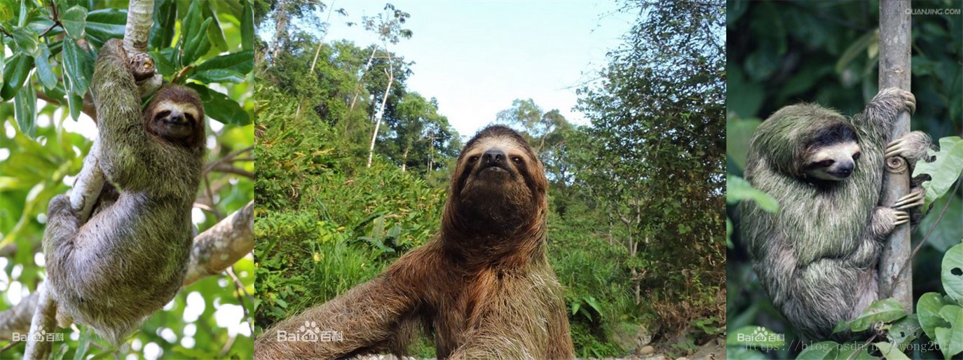
- 森林小稻鼠(
Microryzomys minutus)
数据集介绍
本例使用的物种分布数据集由datasets库函数fetch_species_distributions加载。它有两个参数,其中,data_home指定数据集下载后的存储文件夹,该参数的默认值为None, 表示存储在当前工作目录的scikit_learn_data子目录下。download_if_missing表示如果本地没有可利用的数据,是否从原始网站下载数据。该参数是逻辑型,默认值为True,如果取False, 则在没有找到数据时给出一个错误提示。
函数fetch_species_distributions返回一个Bunch数据对象,它有属性:
- coverages: 数组型,形状[14, 1592, 1212]
它表示在地图网格测量的14个特征的值,其中的缺失值用-9999表示。
- train: 记录数组,形状 (1624,)
它表示数据集的训练点,每个点有三个域:
- train[‘species’]是物种名字
- train[‘dd long’]是经度
- train[‘dd lat’]是纬度
- test: 记录数组,形状 (620,)
它表示数据的检验点,与训练数据格式相同。
- Nx, Ny: 整型
它们分别表示格点的经度(x), 纬度(y)值。
- x_left_lower_corner, y_left_lower_corner: 浮点型
左下角的坐标位置(x, y)
- grid_size: 浮点型
网格上点与点之间的间隔。
实例详解
首先,加载必需的函数模块和库。
# Authors: Peter Prettenhofer <[email protected]>
#          Jake Vanderplas <[email protected]>
#
# License: BSD 3 clause

from __future__ import print_function

from time import time

import numpy as np
import matplotlib.pyplot as plt

from sklearn.datasets.base import Bunch
from sklearn.datasets import fetch_species_distributions
from sklearn.datasets.species_distributions import construct_grids
from sklearn import svm, metrics

# if basemap is available, we'll use it.
# otherwise, we'll improvise later...
try:
    from mpl_toolkits.basemap import Basemap
    basemap = True
except ImportError:
    basemap = False

print(__doc__)
函数 create_species_bunch()
函数create_species_bunch返回一个bunch对象,它描述一个特定物种的信息。该函数包括一个物种名字的参数,这样,使用test/train记录数组提取指定物种的数据。
def create_species_bunch(species_name, train, test, coverages, xgrid, ygrid):
    """Create a bunch with information about a particular organism

    This will use the test/train record arrays to extract the
    data specific to the given species name.
    """
    bunch = Bunch(name=' '.join(species_name.split("_")[:2]))
    species_name = species_name.encode('ascii')
    points = dict(test=test, train=train)

    for label, pts in points.items():
        # choose points associated with the desired species
        pts = pts[pts['species'] == species_name]
        bunch['pts_%s' % label] = pts

        # determine coverage values for each of the training & testing points
        ix = np.searchsorted(xgrid, pts['dd long'])
        iy = np.searchsorted(ygrid, pts['dd lat'])
        bunch['cov_%s' % label] = coverages[:, -iy, ix].T

    return bunch
函数 plot_species_distribution()
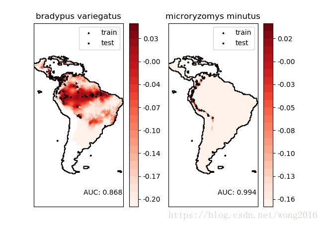
函数plot_species_distribution画出两个物种,即,Bradypus variegatus, Microryzomys minutus的地理分布图。
def plot_species_distribution(species=("bradypus_variegatus_0",
                                       "microryzomys_minutus_0")):
    """
    Plot the species distribution.
    """
    if len(species) > 2:
        print("Note: when more than two species are provided,"
              " only the first two will be used")

    t0 = time()

    # Load the compressed data
    data = fetch_species_distributions()

    # Set up the data grid
    xgrid, ygrid = construct_grids(data)

    # The grid in x,y coordinates
    X, Y = np.meshgrid(xgrid, ygrid[::-1])

    # create a bunch for each species
    BV_bunch = create_species_bunch(species[0],
                                    data.train, data.test,
                                    data.coverages, xgrid, ygrid)
    MM_bunch = create_species_bunch(species[1],
                                    data.train, data.test,
                                    data.coverages, xgrid, ygrid)

    # background points (grid coordinates) for evaluation
    np.random.seed(13)
    background_points = np.c_[np.random.randint(low=0, high=data.Ny,
                                                size=10000),
                              np.random.randint(low=0, high=data.Nx,
                                                size=10000)].T

    # We'll make use of the fact that coverages[6] has measurements at all
    # land points.  This will help us decide between land and water.
    land_reference = data.coverages[6]

    # Fit, predict, and plot for each species.
    for i, species in enumerate([BV_bunch, MM_bunch]):
        print("_" * 80)
        print("Modeling distribution of species '%s'" % species.name)

        # Standardize features
        mean = species.cov_train.mean(axis=0)
        std = species.cov_train.std(axis=0)
        train_cover_std = (species.cov_train - mean) / std

        # Fit OneClassSVM
        print(" - fit OneClassSVM ... ", end='')
        clf = svm.OneClassSVM(nu=0.1, kernel="rbf", gamma=0.5)
        clf.fit(train_cover_std)
        print("done.")

        # Plot map of South America
        plt.subplot(1, 2, i + 1)
        if basemap:
            print(" - plot coastlines using basemap")
            m = Basemap(projection='cyl', llcrnrlat=Y.min(),
                        urcrnrlat=Y.max(), llcrnrlon=X.min(),
                        urcrnrlon=X.max(), resolution='c')
            m.drawcoastlines()
            m.drawcountries()
        else:
            print(" - plot coastlines from coverage")
            plt.contour(X, Y, land_reference,
                        levels=[-9998], colors="k",
                        linestyles="solid")
            plt.xticks([])
            plt.yticks([])

        print(" - predict species distribution")

        # Predict species distribution using the training data
        Z = np.ones((data.Ny, data.Nx), dtype=np.float64)

        # We'll predict only for the land points.
        idx = np.where(land_reference > -9999)
        coverages_land = data.coverages[:, idx[0], idx[1]].T

        pred = clf.decision_function((coverages_land - mean) / std)
        Z *= pred.min()
        Z[idx[0], idx[1]] = pred

        levels = np.linspace(Z.min(), Z.max(), 25)
        Z[land_reference == -9999] = -9999

        # plot contours of the prediction
        plt.contourf(X, Y, Z, levels=levels, cmap=plt.cm.Reds)
        plt.colorbar(format='%.2f')

        # scatter training/testing points
        plt.scatter(species.pts_train['dd long'], species.pts_train['dd lat'],
                    s=2 ** 2, c='black',
                    marker='^', label='train')
        plt.scatter(species.pts_test['dd long'], species.pts_test['dd lat'],
                    s=2 ** 2, c='black',
                    marker='x', label='test')
        plt.legend()
        plt.title(species.name)
        plt.axis('equal')

        # Compute AUC with regards to background points
        pred_background = Z[background_points[0], background_points[1]]
        pred_test = clf.decision_function((species.cov_test - mean) / std)
        scores = np.r_[pred_test, pred_background]
        y = np.r_[np.ones(pred_test.shape), np.zeros(pred_background.shape)]
        fpr, tpr, thresholds = metrics.roc_curve(y, scores)
        roc_auc = metrics.auc(fpr, tpr)
        plt.text(-35, -70, "AUC: %.3f" % roc_auc, ha="right")
        print("\n Area under the ROC curve : %f" % roc_auc)

    print("\ntime elapsed: %.2fs" % (time() - t0))
最后,调用函数plot_species_distribution, 画物种的地理分布图。
plot_species_distribution()
plt.show()
阅读更多精彩内容,请关注微信公众号:统计学习与大数据