源教程：https://rasterio.readthedocs.io/en/latest/quickstart.html

1.使用RasterIO读取栅格数据

# 使用RasterIO读取栅格数据
import rasterio

with rasterio.open('E:/data/L8_BJ_NRG.tif') as ds:
    print('数据信息：')
    print('数据格式：', ds.driver)
    print(f'波段数目：{ds.count}')
    print(f'影像宽度：{ds.width}')
    print(f'影像高度：{ds.height}')
    print(f'地理范围：{ds.bounds}')
    print(f'反射变换参数（六参数模型）：\n {ds.transform}')
    print(f'投影定义：{ds.crs}')  # 获取第一个波段数据，跟GDAL一样索引从1开始
    #  直接获得numpy.ndarray类型的二维数组表示，如果read()函数不加参数，则得到所有波段（第一个维度是波段）
    band1 = ds.read(1)
    print(f'第一波段的最大值：{band1.max()}')
    print(f'第一波段的最小值：{band1.min()}')
    print(f'第一波段的平均值：{band1.mean()}')
    # 根据地理坐标得到行列号
    x, y = (ds.bounds.left + 300, ds.bounds.top - 300)  # 距离左上角东300米，南300米的投影坐标
    row, col = ds.index(x, y)  # 对应的行列号
    print(f'(投影坐标{x}, {y})对应的行列号是({row}, {col})')  # 根据行列号得到地理坐标
    x, y = ds.xy(row, col)  # 中心点的坐标
    print(f'行列号({row}, {col})对应的中心投影坐标是({x}, {y})')  # 那么如何得到对应点左上角的信息
    x, y = (row, col) * ds.transform
    print(f'行列号({row}, {col})对应的左上角投影坐标是({x}, {y})')

 输出结果：

数据信息：
数据格式： GTiff
波段数目：3
影像宽度：7761
影像高度：7881
地理范围：BoundingBox(left=360885.0, bottom=4346085.0, right=593715.0, top=4582515.0)
反射变换参数（六参数模型）：
 | 30.00, 0.00, 360885.00|
| 0.00,-30.00, 4582515.00|
| 0.00, 0.00, 1.00|
投影定义：+init=epsg:32650
第一波段的最大值：65535
第一波段的最小值：0
第一波段的平均值：8122.7403364808
(投影坐标361185.0, 4582215.0)对应的行列号是(10, 10)
行列号(10, 10)对应的中心投影坐标是(361200.0, 4582200.0)
行列号(10, 10)对应的左上角投影坐标是(361185.0, 4582215.0)

2.使用RasterIO创建栅格数据

# 使用RasterIO创建栅格数据
import rasterio
import numpy as np

# 读入的数据是绿，红，近红外波段的合成数据
with rasterio.open('E:/data/L8_BJ_NRG.tif') as src:
    raster = src.read()  # 读取所有波段
    #  源数据的元信息集合（使用字典结构存储了数据格式，数据类型，数据尺寸，投影定义，仿射变换参数等信息）
    profile = src.profile
    # 计算NDVI指数（对除0做特殊处理）
    with np.errstate(divide='ignore', invalid='ignore'):
        ndvi = (raster[2] - raster[1]) / (raster[2] + raster[1])
        ndvi[ndvi == np.inf] = 0
        ndvi = np.nan_to_num(ndvi)  # 写入数据
        profile.update(dtype=ndvi.dtype, count=1)
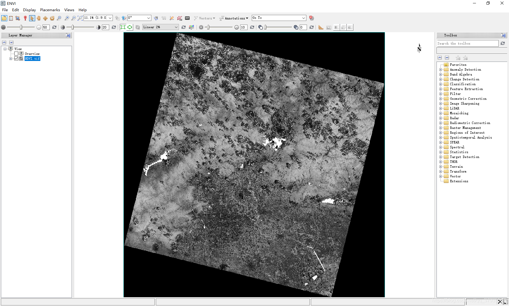
    with rasterio.open('E:/data/NDVI.tif', mode='w', **profile) as dst:
        dst.write(ndvi, 1)

 在ENVI中打开生成的NDVI.tif文件：