《机器学习实战3》

2017.3.6
第三章《决策树的构造》

思维导图：

在这里插入图片描述

1、基本算法原理

理解数据集中蕴含的知识信息，根据特征进行划分，形成一定的规则，最终形成规则树，按照这个规则树即可以将数据分类出来。
优点：计算复杂度不高，输出结果易于理解，对中间值的缺失不敏感，可以处理不相关特
征数据。
缺点：可能会产生过度匹配问题
适用数据类型：数值型和标称型<>

2、构造一颗决策树的流程：

检测数据集中每一个子项的属性是否属于同一类

     if so return 类标签；
     else
         寻找划分数据集的最好特征
         划分数据集
         创建分支结点
            for 每个划分的子集
                调用createBranch并增加返回结果到分支结点中
         return 分支结点

3、决策树的一般流程：

(1)收集数据：可以使用任何方法。
(2)准备数据：决策树算法只适用于标称型数据，数值数据必须离散化
(3)分析数据：树构造完成之后检查是否符合预期
(4)训练算法：构造树的数据结构
(5)测试算法：计算错误率

1、信息增益

划分数据集前后信息发生的变化就是增益，活动的信息增益最高的特征就是最好的选择。换句话说，信息增益以及“熵”(entropy)就是决策树的属性选择函数。熵就是数据集中信息的无序性的体现，这和其他领域中熵的意义是一样的。
书里用到的熵的计算方法如下：
在这里插入图片描述
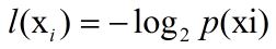
其中p(xi)是选择分类的概率
还有所有类别的信息期望值：

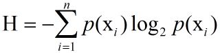
完成上述计算熵的代码如下：

def calcShannonEnt(dataSet):
    numEntries = len(dataSet)
    labelCounts = {}
    for featVec in dataSet: #the the number of unique elements and their occurance
        currentLabel = featVec[-1]
        if currentLabel not in labelCounts.keys(): labelCounts[currentLabel] = 0
        labelCounts[currentLabel] += 1
    shannonEnt = 0.0
    for key in labelCounts:
        prob = float(labelCounts[key])/numEntries
        shannonEnt -= prob * log(prob,2) #log base 2
    return shannonEnt

2、划分数据集

划分数据集的关键在于寻找恰当的特征值来进行划分。我们需要尝试数据集中的每一个特征值的划分并且计算该划分的熵。通过比较得出最终的结果。
根据给定特征值划分数据集：

def splitDataSet(dataSet, axis, value):
    retDataSet = []
    for featVec in dataSet:
        if featVec[axis] == value:
            #把特征值去除
            reducedFeatVec = featVec[:axis]     
            reducedFeatVec.extend(featVec[axis+1:])
            retDataSet.append(reducedFeatVec)
    return retDataSet

依次计算数据集中去除某一特征值余下集合的熵，取得熵增最大值的特征值，就是划分数据集的特征值。

def chooseBestFeatureToSplit(dataSet):
    numFeatures = len(dataSet[0]) - 1      #the last column is used for the labels
    baseEntropy = calcShannonEnt(dataSet)
    bestInfoGain = 0.0; bestFeature = -1
    for i in range(numFeatures):        #iterate over all the features
        featList = [example[i] for example in dataSet]#create a list of all the examples of this feature
        uniqueVals = set(featList)       #get a set of unique values
        newEntropy = 0.0
        for value in uniqueVals:
            subDataSet = splitDataSet(dataSet, i, value)
            prob = len(subDataSet)/float(len(dataSet))
            newEntropy += prob * calcShannonEnt(subDataSet)     
        #calculate the info gain; ie reduction in entropy
        infoGain = baseEntropy - newEntropy    
        #compare this to the best gain so far 
        if (infoGain > bestInfoGain): 
            #if better than current best, set to best      
            bestInfoGain = infoGain         
            bestFeature = i
     #returns an integer
    return bestFeature

3、递归构造决策树

结合书上的例子，我们可以非常直观的看到如何构建决策树。其实就是每一步不断应用上述方法划分数据集的过程。

递归终止的条件是：已经遍历完数据集中的所有属性或者每一个分支下的所有实例都具有相同的分类。

但是如果数据集中所有的属性都已经被划分过，仍然有某个分支下的实例不具有相同的分类怎么办呢？书上给出的方法是多数表决，也是非常合情合理的选择。

def majorityCnt(classList):
    classCount={}
    for vote in classList:
        if vote not in classCount.keys(): classCount[vote] = 0
        classCount[vote] += 1
    sortedClassCount = sorted(classCount.iteritems(), key=operator.itemgetter(1), reverse=True)
    return sortedClassCount[0][0]

这和之前kNN算法的投票部分非常相似。
接下来就是根据上述方法的创建决策树代码：

def createTree(dataSet,labels):
    classList = [example[-1] for example in dataSet]
    #当某一分支下所有数据的类型相同停止
    if classList.count(classList[0]) == len(classList): 
        return classList[0]
    #当数据集中所有属性已经被划分完毕时结束，这里将上述两种情况合二为一了，不管最后分支下的实例是不是都属于同一类，都进行投票。
    if len(dataSet[0]) == 1: 
        return majorityCnt(classList)
    bestFeat = chooseBestFeatureToSplit(dataSet)
    bestFeatLabel = labels[bestFeat]
    myTree = {bestFeatLabel:{}}
    del(labels[bestFeat])
    featValues = [example[bestFeat] for example in dataSet]
    uniqueVals = set(featValues)
    for value in uniqueVals:
        #python中传入的参数为列表是使传入引用，所以这里复制一下
        subLabels = labels[:]       
        myTree[bestFeatLabel][value] = createTree(splitDataSet(dataSet, bestFeat, value),subLabels)
    return myTree

在这里插入图片描述

4、绘制决策树

matplotlib提供了一个注解工具annotations,跟matlab中的非常相似[不过个人认为matlab画图操作起来更加方便]，他是一个很强大的工具。
首先我们先绘制决策树的一个节点:

# coding=utf-8
import matplotlib.pyplot as plt

decisionNode = dict(boxstyle="sawtooth", fc="0.8")
leafNode = dict(boxstyle="round4", fc="0.8")
arrow_args = dict(arrowstyle="<-")

def plotNode(nodeTxt, centerPt, parentPt, nodeType):
    createPlot.ax1.annotate(nodeTxt, xy=parentPt,  xycoords='axes fraction',xytext=centerPt, textcoords='axes fraction',va="center", ha="center", bbox=nodeType, arrowprops=arrow_args )

def createPlot():
    fig = plt.figure(1, facecolor='white')
    plt.xlabel('abs')
    plt.xlabel('c')
    fig.clf()
    createPlot.ax1 = plt.subplot(111, frameon=False) 
    plotNode('a decision node', (0.5, 0.1), (0.1, 0.5), decisionNode)
    plotNode('a leaf node', (0.8, 0.1), (0.3, 0.8), leafNode)
    plt.show()

在powershell中运行上述结果得到以下图片
在这里插入图片描述
然后我们要构造出注解树：
这里自然而然想到用迭代开始构造每一个节点的情况。事实上也确实如此。
先计算注解树的深度以及叶子节点个数，方便迭代的开始和结束

def getNumLeafs(myTree):
    numLeafs = 0
    firstStr = myTree.keys()[0]
    secondDict = myTree[firstStr]
    for key in secondDict.keys():
        #查看当前节点是否已经是叶子节点，如果不是则要再次迭代
        if type(secondDict[key]).__name__=='dict':
            numLeafs += getNumLeafs(secondDict[key])
        else:   numLeafs +=1
    return numLeafs

def getTreeDepth(myTree):
    maxDepth = 0
    firstStr = myTree.keys()[0]
    secondDict = myTree[firstStr]
    for key in secondDict.keys():
        #查看当前节点是否已经是叶子节点，如果不是则要再次迭代
        if type(secondDict[key]).__name__=='dict':
            thisDepth = 1 + getTreeDepth(secondDict[key])
        else:   thisDepth = 1
        if thisDepth > maxDepth: maxDepth = thisDepth
    return maxDepth

下面就是画出注解树的主函数：

def plotMidText(cntrPt, parentPt, txtString):
    xMid = (parentPt[0]-cntrPt[0])/2.0 + cntrPt[0]
    yMid = (parentPt[1]-cntrPt[1])/2.0 + cntrPt[1]
    createPlot.ax1.text(xMid, yMid, txtString, va="center", ha="center", rotation=30)

def plotTree(myTree, parentPt, nodeTxt):#if the first key tells you what feat was split on
    numLeafs = getNumLeafs(myTree)  #this determines the x width of this tree
    depth = getTreeDepth(myTree)
    firstStr = myTree.keys()[0]     #the text label for this node should be this
    cntrPt = (plotTree.xOff + (1.0 + float(numLeafs))/2.0/plotTree.totalW, plotTree.yOff)
    plotMidText(cntrPt, parentPt, nodeTxt)
    plotNode(firstStr, cntrPt, parentPt, decisionNode)
    secondDict = myTree[firstStr]
    plotTree.yOff = plotTree.yOff - 1.0/plotTree.totalD
    for key in secondDict.keys():
        if type(secondDict[key]).__name__=='dict':#test to see if the nodes are dictonaires, if not they are leaf nodes   
            plotTree(secondDict[key],cntrPt,str(key))        #recursion
        else:   #it's a leaf node print the leaf node
            plotTree.xOff = plotTree.xOff + 1.0/plotTree.totalW
            plotNode(secondDict[key], (plotTree.xOff, plotTree.yOff), cntrPt, leafNode)
            plotMidText((plotTree.xOff, plotTree.yOff), cntrPt, str(key))
    plotTree.yOff = plotTree.yOff + 1.0/plotTree.totalD
#if you do get a dictonary you know it's a tree, and the first element will be another dict

def createPlot(inTree):
    fig = plt.figure(1, facecolor='white')
    fig.clf()
    axprops = dict(xticks=[], yticks=[])
    createPlot.ax1 = plt.subplot(111, frameon=False, **axprops)    #no ticks
    #createPlot.ax1 = plt.subplot(111, frameon=False) #ticks for demo puropses 
    plotTree.totalW = float(getNumLeafs(inTree))
    plotTree.totalD = float(getTreeDepth(inTree))
    plotTree.xOff = -0.5/plotTree.totalW; plotTree.yOff = 1.0;
    plotTree(inTree, (0.5,1.0), '')
    plt.show()

在这里插入图片描述

5、决策树算法应用

眼科医生根据病人的情况决定给病人选配哪一种隐形眼镜。这是一个专家系统的问题，可以用决策树来进行分类得出分类指标。

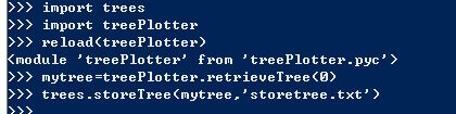
由于生成决策树很费时，我们没有必要每次使用决策树都重新生成一个决策树,书中介绍了pickle序列化的方法存储一棵已经生成了的决策树。

pickle模块的基本用法如下用法。
使用pickle模块存储决策树：

def storeTree(inputTree,filename):
    import pickle
    fw = open(filename,'w')
    pickle.dump(inputTree,fw)
    fw.close()

def grabTree(filename):
    import pickle
    fr = open(filename)
    return pickle.load(fr)

在这里插入图片描述
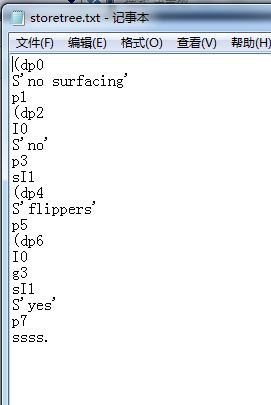
存储形式如下:

实现步骤

收集数据：提供文本文件
准备数据：解析tab键分割的数据行
分析数据：使用createPlot()函数绘制最终的树形图
训练算法：使用createTree()函数
测试算法：根据实际情况测试算法是否可以正确分类
使用算法：存储决策树结构，下次直接使用