AlexNet是最早的现代神经网络,是由(亚历克斯)等人在2012年的ImageNet比赛中发明的一种卷积神经网络,并以此模型拿到了冠军。它证明了CNN在复杂模型下的有效性,使用GPU使训练在可接受的时间范围内得到结果,推动了有监督深度学习的发展。
AlexNet网络结构如下图所示,包括8个带权层;前5层是卷积层,剩下3层是全连接层最后一个全连接层输出到一个1000维的使用SoftMax层,其产生一个覆盖1000类标签的分布。
第一个卷积层利用96个大小为11 * 11 * 3,步长为4个像素的核(两个GPU各48个),对大小为224 * 224 * 3的输入图像进行卷积。第二个卷积层需要将第一个卷积层的输出作为自己的输入,且利用大小为5 * 5 * 48的核对其进行滤波(48为输入图像的通道数)。第三,第四和第五个卷积层彼此相连,没有任何介于中间的池化层。第三个卷积层有384个大小为3×3×256的核被连接到第二个卷积层的(归一化的,池化的)输出。第四个卷积层拥有384个大小为3×3×192的核,第五个卷积层拥有256个大小为3×3×192的核。全连接层都各有4096个神经元。

第二,四,五卷积层的核只连接到同一个显卡上的前一个卷积层,第三个卷积层的核连接到第二个卷积层中的所有核映射上,并且将两块显卡的通道进行合并。全连接层中的神经元被连接到前一层中的所有的神经元上,其中第1个全连接层需要处理通道合并(两个显卡),AlexNet最后的输出类目是1000个,所以其输出为1000 ..
代码如下所示:
from datetime import datetime
import math,time
import tensorflow as tf
batch_size = 32
num_bathes = 100
'''
获取tensor信息
'''
def print_tensor_info(tensor):
print("tensor name:",tensor.op.name,"-tensor shape:",tensor.get_shape().as_list())
'''
计算每次迭代消耗时间
session:TensorFlow的Session
target:需要评测的运算算子
info_string:测试的名称
'''
def time_tensorflow_run(session,target,info_string):
#前10次迭代不计入时间消耗
num_step_burn_in = 10
total_duration = 0.0
total_duration_squared = 0.0
for i in range(num_bathes + num_step_burn_in):
start_time = time.time()
_ = session.run(target)
duration = time.time() - start_time
if i >= num_step_burn_in:
if not i % 10 :
print("%s:step %d,duration=%.3f"%(datetime.now(),i-num_step_burn_in,duration))
total_duration += duration
total_duration_squared += duration * duration
#计算消耗时间的平均差
mn = total_duration / num_bathes
#计算消耗时间的标准差
vr = total_duration_squared / num_bathes - mn * mn
std = math.sqrt(vr)
print("%s:%s across %d steps,%.3f +/- %.3f sec / batch"%(datetime.now(),info_string,num_bathes,
mn,std))
#主函数
def run_bechmark():
with tf.Graph().as_default():
image_size = 224
#以高斯分布产生一些图片
images = tf.Variable(tf.random_normal([batch_size,image_size,image_size,3],
dtype=tf.float32,stddev=0.1))
output,parameters = inference(images)
init = tf.global_variables_initializer()
sess = tf.Session()
sess.run(init)
time_tensorflow_run(sess,output,"Forward")
objective = tf.nn.l2_loss(output)
grad = tf.gradients(objective,parameters)
time_tensorflow_run(sess,grad,"Forward-backward")
def inference(images):
#定义参数
parameters = []
#第一层卷积层
with tf.name_scope("conv1") as scope:
#设置卷积核11×11,3通道,64个卷积核
kernel1 = tf.Variable(tf.truncated_normal([11,11,3,64],mean=0,stddev=0.1,
dtype=tf.float32),name="weights")
#卷积,卷积的横向步长和竖向补偿都为4
conv = tf.nn.conv2d(images,kernel1,[1,4,4,1],padding="SAME")
#初始化偏置
biases = tf.Variable(tf.constant(0,shape=[64],dtype=tf.float32),trainable=True,name="biases")
bias = tf.nn.bias_add(conv,biases)
#RELU激活函数
conv1 = tf.nn.relu(bias,name=scope)
#输出该层的信息
print_tensor_info(conv1)
#统计参数
parameters += [kernel1,biases]
#lrn处理
lrn1 = tf.nn.lrn(conv1,4,bias=1,alpha=1e-3/9,beta=0.75,name="lrn1")
#最大池化
pool1 = tf.nn.max_pool(lrn1,ksize=[1,3,3,1],strides=[1,2,2,1],padding="VALID",name="pool1")
print_tensor_info(pool1)
#第二层卷积层
with tf.name_scope("conv2") as scope:
#初始化权重
kernel2 = tf.Variable(tf.truncated_normal([5,5,64,192],dtype=tf.float32,stddev=0.1)
,name="weights")
conv = tf.nn.conv2d(pool1,kernel2,[1,1,1,1],padding="SAME")
#初始化偏置
biases = tf.Variable(tf.constant(0,dtype=tf.float32,shape=[192])
,trainable=True,name="biases")
bias = tf.nn.bias_add(conv,biases)
#RELU激活
conv2 = tf.nn.relu(bias,name=scope)
print_tensor_info(conv2)
parameters += [kernel2,biases]
#LRN
lrn2 = tf.nn.lrn(conv2,4,1.0,alpha=1e-3/9,beta=0.75,name="lrn2")
#最大池化
pool2 = tf.nn.max_pool(lrn2,[1,3,3,1],[1,2,2,1],padding="VALID",name="pool2")
print_tensor_info(pool2)
#第三层卷积层
with tf.name_scope("conv3") as scope:
#初始化权重
kernel3 = tf.Variable(tf.truncated_normal([3,3,192,384],dtype=tf.float32,stddev=0.1)
,name="weights")
conv = tf.nn.conv2d(pool2,kernel3,strides=[1,1,1,1],padding="SAME")
biases = tf.Variable(tf.constant(0.0,shape=[384],dtype=tf.float32),trainable=True,name="biases")
bias = tf.nn.bias_add(conv,biases)
#RELU激活层
conv3 = tf.nn.relu(bias,name=scope)
parameters += [kernel3,biases]
print_tensor_info(conv3)
#第四层卷积层
with tf.name_scope("conv4") as scope:
#初始化权重
kernel4 = tf.Variable(tf.truncated_normal([3,3,384,256],stddev=0.1,dtype=tf.float32),
name="weights")
#卷积
conv = tf.nn.conv2d(conv3,kernel4,strides=[1,1,1,1],padding="SAME")
biases = tf.Variable(tf.constant(0.0,dtype=tf.float32,shape=[256]),trainable=True,name="biases")
bias = tf.nn.bias_add(conv,biases)
#RELU激活
conv4 = tf.nn.relu(bias,name=scope)
parameters += [kernel4,biases]
print_tensor_info(conv4)
#第五层卷积层
with tf.name_scope("conv5") as scope:
#初始化权重
kernel5 = tf.Variable(tf.truncated_normal([3,3,256,256],stddev=0.1,dtype=tf.float32),
name="weights")
conv = tf.nn.conv2d(conv4,kernel5,strides=[1,1,1,1],padding="SAME")
biases = tf.Variable(tf.constant(0.0,dtype=tf.float32,shape=[256]),name="biases")
bias = tf.nn.bias_add(conv,biases)
#REUL激活层
conv5 = tf.nn.relu(bias)
parameters += [kernel5,bias]
#最大池化
pool5 = tf.nn.max_pool(conv5,[1,3,3,1],[1,2,2,1],padding="VALID",name="pool5")
print_tensor_info(pool5)
#第六层全连接层
pool5 = tf.reshape(pool5,(-1,6*6*256))
weight6 = tf.Variable(tf.truncated_normal([6*6*256,4096],stddev=0.1,dtype=tf.float32),
name="weight6")
ful_bias1 = tf.Variable(tf.constant(0.0,dtype=tf.float32,shape=[4096]),name="ful_bias1")
ful_con1 = tf.nn.relu(tf.add(tf.matmul(pool5,weight6),ful_bias1))
#第七层第二层全连接层
weight7 = tf.Variable(tf.truncated_normal([4096,4096],stddev=0.1,dtype=tf.float32),
name="weight7")
ful_bias2 = tf.Variable(tf.constant(0.0,dtype=tf.float32,shape=[4096]),name="ful_bias2")
ful_con2 = tf.nn.relu(tf.add(tf.matmul(ful_con1,weight7),ful_bias2))
#
#第八层第三层全连接层
weight8 = tf.Variable(tf.truncated_normal([4096,1000],stddev=0.1,dtype=tf.float32),
name="weight8")
ful_bias3 = tf.Variable(tf.constant(0.0,dtype=tf.float32,shape=[1000]),name="ful_bias3")
ful_con3 = tf.nn.relu(tf.add(tf.matmul(ful_con2,weight8),ful_bias3))
#softmax层
weight9 = tf.Variable(tf.truncated_normal([1000,10],stddev=0.1),dtype=tf.float32,name="weight9")
bias9 = tf.Variable(tf.constant(0.0,shape=[10]),dtype=tf.float32,name="bias9")
output_softmax = tf.nn.softmax(tf.matmul(ful_con3,weight9)+bias9)
return output_softmax,parameters
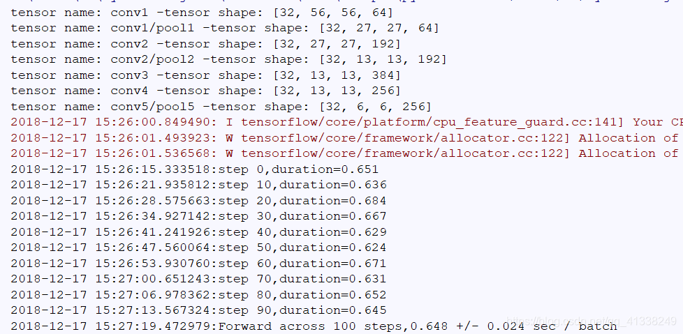
if __name__ == "__main__":
run_bechmark()运行结果如下所示:
AlexNet之所以能够取得成功的原因如下。
- 采用非线性激活函数RELU
正切和乙状结肠函数在输入非常大或者非常小时,输出结果变化不大,容易饱和这类非线性函数随着网络层次的增加引起梯度弥散现象,即顶层误差较大;逐层递减误差传递过程中,底层误差很小,导致深度网络底层权值更新量很小,使深层网络出现局部最优.ReLU为扭曲线性函数,不仅比饱和函数训练更快,而且保留了非线性的表达能力,可以训练更深层的网络。
- 采用数据增强和漏失防止过拟合
数据增强是采用图像平移和翻转来生成更多的训练图像,从256×256的图像中提取随机的224 * 224的碎片,并在这些提取的碎片上训练网络,这就是输入图像是224 * 224 * 3维的原因。扩大了训练集规模,达到2048倍(32×32×2 = 2048)。此外,调整图像的RGB像素值,在整个ImageNet训练集的RGB像素值集合中执行PCA,通过对每个训练图像,增加已有主成分RGB值,在不改变对象核心特征的基础上,增加光照强度和颜色变化的因素,间接增加训练集数量。
Dropout是以0.5的概率将每个隐层神经元的输出设置为零,使这些神经元不参与前向传播,也不参与反向传播,只有被选中参与连接的节点上进行正向和反向传播,神经网络在输入数据时会尝试不同的结构,但是结构之间共享权重。这种技术降低了神经元之间互适应关系,而被迫学习更为健壮的特征。
- 采用GPU实现
AlexNet网络采用了并行化GPU进行训练,在每个GPU中放置一半核(或神经元),GPU间的通讯只在某些层进行。采用交叉验证,精确地调整通信量,直到它的计算量可接受。