数据预处理
不同于导入 scikit-learn 自有乳腺癌数据集,采用 pandas 读取下载的数据集。
# 载入数据
from sklearn.datasets import load_breast_cancer

cancer = load_breast_cancer()
X = cancer.data
y = cancer.target
print('data shape: {0}; no. positive: {1}; no. negative: {2}'.format(
    X.shape, y[y==1].shape[0], y[y==0].shape[0]))
data shape: (569, 30); no. positive: 357; no. negative: 212
注意:自有数据集中 diagnosis 已经是0,1形式的 int 型数据。
import pandas as pd
import numpy as np
import matplotlib.pyplot as plt
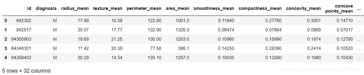
data = pd.read_csv(r'D:\machinelearningDatasets\BreastCancerLR\Breast cancer.csv')
X = data.iloc[:,2:31]
y = data.iloc[:,1:2]
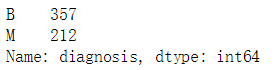
y.diagnosis.value_counts()
y = y.values.ravel()
数据标准化:
sklearn.preprocessing.MinMaxScaler
Transforms features by scaling each feature to a given range.
from sklearn.preprocessing import MinMaxScaler
scaler = MinMaxScaler()
X = scaler.fit_transform(X)
划分数据集:
from sklearn.model_selection import train_test_split

X_train, X_test, y_train, y_test = train_test_split(X, y, test_size=0.2)
高斯核函数(rbf)
from sklearn.svm import SVC

clf = SVC(C=1.0, kernel='rbf')
clf.fit(X_train, y_train)
train_score = clf.score(X_train, y_train)
test_score = clf.score(X_test, y_test)
print('train score: {0}; test score: {1}'.format(train_score, test_score))
train score: 0.9538461538461539; test score: 0.9649122807017544
拟合非常好!
不对数据标准化时:
train score: 1.0; test score: 0.631578947368421
训练集分数接近满分,而验证集评分很低,典型的过拟合现象。此时优化gamma也可使评分达到0.950。
模型优化:
import sys
sys.path.append(r'C:\Users\Qiuyi\Desktop\scikit-learn code\code\common')

from utils import plot_param_curve
from sklearn.model_selection import GridSearchCV

gammas = np.linspace(0, 0.001, 50)
C = [1, 10, 100,1000]
param_grid = {'gamma': gammas, 'C':C}

clf = GridSearchCV(SVC(), param_grid, cv=5, return_train_score=True)
clf.fit(X, y)
print("best param: {0}\nbest score: {1}".format(clf.best_params_,
                                                clf.best_score_))
best param: {‘C’: 1000, ‘gamma’: 0.0008979591836734694}
best score: 0.9789103690685413
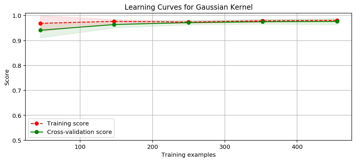
绘制学习曲线:
import time
from utils import plot_learning_curve
from sklearn.model_selection import ShuffleSplit

cv = ShuffleSplit(n_splits=10, test_size=0.2, random_state=0)
title = 'Learning Curves for Gaussian Kernel'

start = time.clock()
plt.figure(figsize=(10, 4), dpi=144)
plot_learning_curve(plt, SVC(C=1000, kernel='rbf', gamma=0.0008979591836734694),
                    title, X, y, ylim=(0.5, 1.01), cv=cv)

print('elaspe: {0:.6f}'.format(time.clock()-start))
elaspe: 0.340826
多项式核函数(poly)
简单测试一下,运行明显比高斯核函数慢一些。
from sklearn.svm import SVC

clf = SVC(C=1.0, kernel='poly', degree=2)
clf.fit(X_train, y_train)
train_score = clf.score(X_train, y_train)
test_score = clf.score(X_test, y_test)
print('train score: {0}; test score: {1}'.format(train_score, test_score))
train score: 0.967032967032967; test score: 0.9473684210526315
拟合情况比较好!
绘制学习曲线:
import time
from utils import plot_learning_curve
from sklearn.model_selection import ShuffleSplit

cv = ShuffleSplit(n_splits=5, test_size=0.2, random_state=0)
title = 'Learning Curves with degree={0}'
degrees = [1, 2]

start = time.clock()
plt.figure(figsize=(12, 4), dpi=144)
for i in range(len(degrees)):
    plt.subplot(1, len(degrees), i + 1)
    plot_learning_curve(plt, SVC(C=1.0, kernel='poly', degree=degrees[i]),
                        title.format(degrees[i]), X, y, ylim=(0.8, 1.01), cv=cv, n_jobs=-1)

print('elaspe: {0:.6f}'.format(time.clock()-start))
elaspe: 431.939271
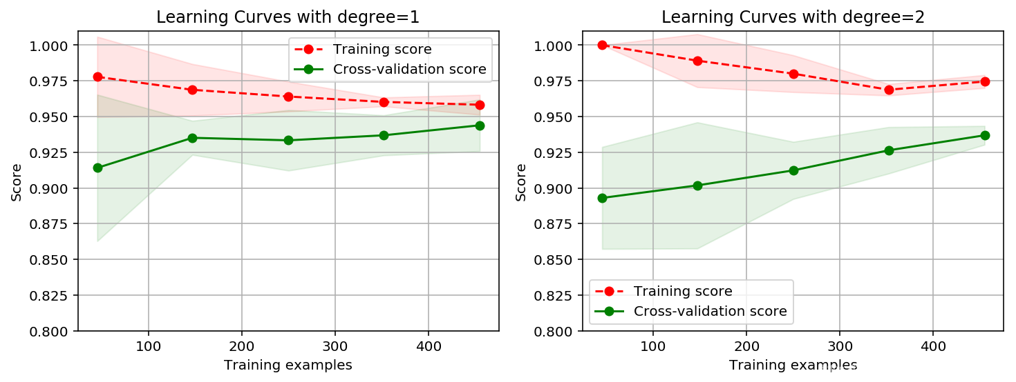
计算代价非常高!
一阶多项式核函数分数偏高一些。但仍不如高斯核函数。
多项式 LinearSVC
LinearSVC() 与 SVC(kernel=‘linear’) 的区别:
- LinearSVC() 最小化 hinge loss的平方,
SVC(kernel=‘linear’) 最小化 hinge loss; - LinearSVC() 使用 one-vs-rest 处理多类问题,
SVC(kernel=‘linear’) 使用 one-vs-one 处理多类问题; - LinearSVC() 使用 liblinear 执行,
SVC(kernel=‘linear’)使用 libsvm 执行; - LinearSVC() 可以选择正则项和损失函数,
SVC(kernel=‘linear’)使用默认设置。
一句话,大规模线性可分问题上 LinearSVC 更快。
from sklearn.svm import LinearSVC
from sklearn.preprocessing import PolynomialFeatures
from sklearn.preprocessing import MinMaxScaler
from sklearn.pipeline import Pipeline

def create_model(degree=2, **kwarg):
    polynomial_features = PolynomialFeatures(degree=degree, include_bias=False)
    scaler = MinMaxScaler()
    linear_svc = LinearSVC(**kwarg)
    pipeline = Pipeline([("polynomial_features", polynomial_features),
                         ("scaler", scaler),
                         ("linear_svc", linear_svc)])
    return pipeline

clf = create_model(penalty='l1', dual=False)
clf.fit(X_train, y_train)
train_score = clf.score(X_train, y_train)
test_score = clf.score(X_test, y_test)
print('train score: {0}; test score: {1}'.format(train_score, test_score))
train score: 0.9824175824175824; test score: 0.9649122807017544
import time
from utils import plot_learning_curve
from sklearn.model_selection import ShuffleSplit

cv = ShuffleSplit(n_splits=5, test_size=0.2, random_state=0)
title = 'Learning Curves for LinearSVC with Degree={0}'
degrees = [1, 2]

start = time.clock()
plt.figure(figsize=(12, 4), dpi=144)
for i in range(len(degrees)):
    plt.subplot(1, len(degrees), i + 1)
    plot_learning_curve(plt, create_model(penalty='l1', dual=False, degree=degrees[i]),
                        title.format(degrees[i]), X, y, ylim=(0.8, 1.01), cv=cv)

print('elaspe: {0:.6f}'.format(time.clock()-start))
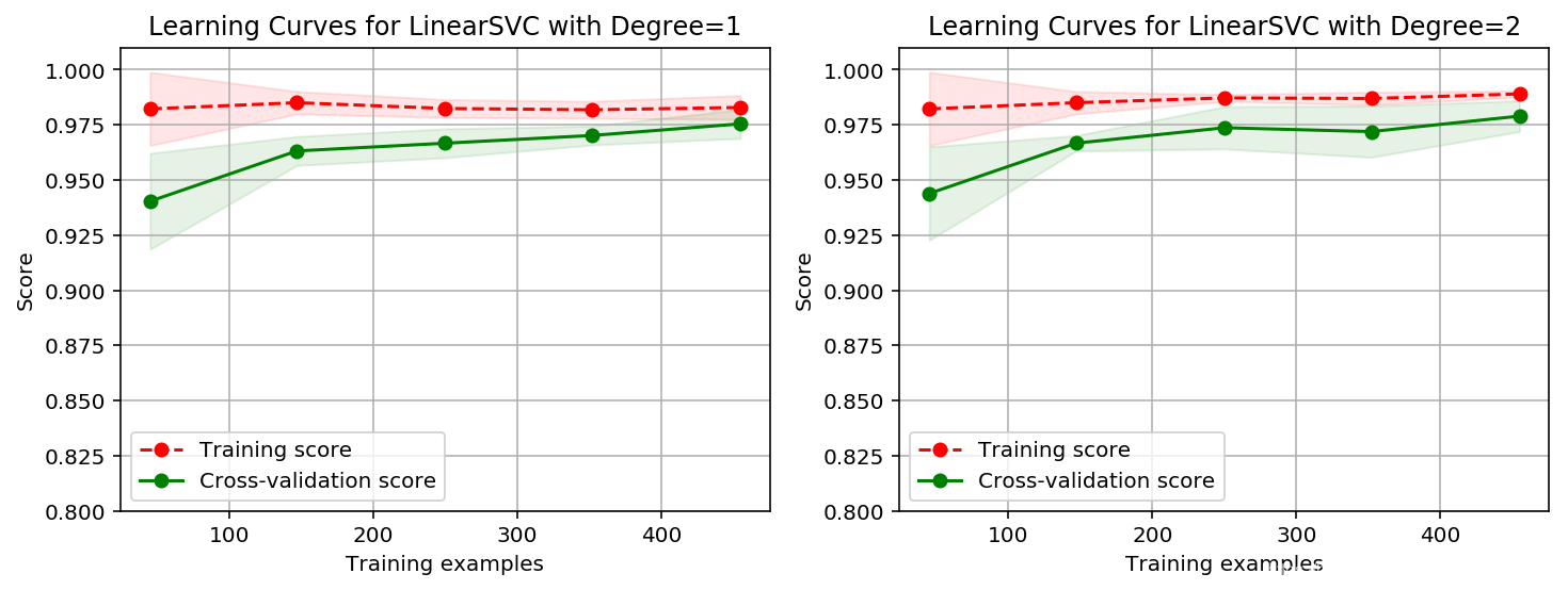
拟合情况略差于高斯核函数,但好于多项式核函数!关键是比较快!
参考:
common\utils
第3章 plot_learning_curve 绘制学习曲线
注意事项:
必须 values.ravel() ,否则:
C:\Python36\lib\site-packages\sklearn\utils\validation.py:578: DataConversionWarning: A column-vector y was passed when a 1d array was expected. Please change the shape of y to (n_samples, ), for example using ravel().
y = column_or_1d(y, warn=True)
GridSearchCV 利用 mean_train_score 等参数时,必须有 return_train_score=True ,否则会报错。
plot_param_curve()
train_scores_mean = cv_results[‘mean_train_score’]
train_scores_std = cv_results[‘std_train_score’]
test_scores_mean = cv_results[‘mean_test_score’]
test_scores_std = cv_results[‘std_test_score’]