在简单易学的机器学习算法——马尔可夫链蒙特卡罗方法MCMC中简单介绍了马尔可夫链蒙特卡罗MCMC方法的基本原理,介绍了Metropolis采样算法的基本过程,这一部分,主要介绍Metropolis-Hastings采样算法,Metropolis-Hastings采样算法也是基于MCMC的采样算法,是Metropolis采样算法的推广形式。
一、Metropolis-Hastings算法的基本原理
1、Metropolis-Hastings算法的基本原理
与Metropolis采样算法类似,假设需要从目标概率密度函数
p(θ)
中进行采样,同时,
θ
满足
−∞<θ<∞
。Metropolis-Hastings采样算法根据马尔可夫链去生成一个序列:
θ(1)→θ(2)→⋯θ(t)→
其中,
θ(t)
表示的是马尔可夫链在第
t
代时的状态。
在Metropolis-Hastings采样算法的过程中,首先初始化状态值
θ(1)
,然后利用一个已知的分布
q(θ∣θ(t−1))
生成一个新的候选状态
θ(∗)
,随后根据一定的概率选择接受这个新值,或者拒绝这个新值,与Metropolis采样算法不同的是,在Metropolis-Hastings采样算法中,概率为:
α=min⎛⎝⎜1,p(θ(∗))p(θ(t−1))q(θ(t−1)∣θ(∗))q(θ(∗)∣θ(t−1))⎞⎠⎟
这样的过程一直持续到采样过程的收敛,当收敛以后,样本
θ(t)
即为目标分布
p(θ)
中的样本。
2、Metropolis-Hastings采样算法的流程
基于以上的分析,可以总结出如下的Metropolis-Hastings采样算法的流程:
- 初始化时间
t=1
- 设置
u
的值,并初始化初始状态
θ(t)=u
- 重复以下的过程:
- 令
t=t+1
- 从已知分布
q(θ∣θ(t−1))
中生成一个候选状态
θ(∗)
- 计算接受的概率:
α=min(1,p(θ(∗))p(θ(t−1))q(θ(t−1)∣θ(∗))q(θ(∗)∣θ(t−1)))
- 从均匀分布
Uniform(0,1)
生成一个随机值
a
- 如果
a⩽α
,接受新生成的值:
θ(t)=θ(∗)
;否则:
θ(t)=θ(t−1)
- 直到
t=T
3、Metropolis-Hastings采样算法的解释
与Metropolis采样算法类似,要证明Metropolis-Hastings采样算法的正确性,最重要的是要证明构造的马尔可夫过程满足如上的细致平稳条件,即:
π(i)Pi,j=π(j)Pj,i
对于上面所述的过程,分布为
p(θ)
,从状态
i
转移到状态
j
的转移概率为:
Pi,j=αi,j⋅Qi,j
其中,
Qi,j
为上述已知的分布,
Qi,j
为:
Qi,j=q(θ(j)∣θ(i))
在Metropolis-Hastings采样算法中,并不要求像Metropolis采样算法中的已知分布为对称的。
接下来,需要证明在Metropolis-Hastings采样算法中构造的马尔可夫链满足细致平稳条件。
因此,通过以上的方法构造出来的马尔可夫链是满足细致平稳条件的。
4、实验1
如前文的Metropolis采样算法,假设需要从柯西分布中采样数据,我们利用Metropolis-Hastings采样算法来生成样本,其中,柯西分布的概率密度函数为:
f(θ)=1π(1+θ2)
那么,根据上述的Metropolis-Hastings采样算法的流程,接受概率
α
的值为:
α=min⎛⎝⎜⎜1,1+[θ(t)]21+[θ(∗)]2q(θ(t)∣θ(∗))q(θ(∗)∣θ(t))⎞⎠⎟⎟
若已知的分布符合条件独立性,则
q(θ(t)∣θ(∗))q(θ(∗)∣θ(t))=1
此时,与Metropolis采样算法一致。
二、多变量分布的采样
上述的过程中,都是针对的是单变量分布的采样,对于多变量的采样,Metropolis-Hastings采样算法通常有以下的两种策略:
- Blockwise Metropolis-Hastings采样
- Componentwise Metropolis-Hastings采样
1、Blockwise Metropolis-Hastings采样
对于BlockWise Metropolis-Hastings采样算法,在选择已知分布时,需要选择与目标分布具有相同维度的分布。针对上述的更新策略,在BlockWise Metropolis-Hastings采样算法中采用的是向量的更新策略,即:
Θ=(θ1,θ2,⋯,θN)
。因此,算法流程为:
- 初始化时间
t=1
- 设置
u
的值,并初始化初始状态
Θ(t)=u
- 重复以下的过程:
- 令
t=t+1
- 从已知分布
q(Θ∣Θ(t−1))
中生成一个候选状态
Θ(∗)
- 计算接受的概率:
α=min(1,p(Θ(∗))p(Θ(t−1))q(Θ(t−1)∣Θ(∗))q(Θ(∗)∣Θ(t−1)))
- 从均匀分布
Uniform(0,1)
生成一个随机值
a
- 如果
a⩽α
,接受新生成的值:
Θ(t)=Θ(∗)
;否则:
Θ(t)=Θ(t−1)
- 直到
t=T
2、Componentwise Metropolis-Hastings采样
对于上述的BlockWise Metropolis-Hastings采样算法,有时很难找到与所要采样的分布具有相同维度的分布,因此可以采用Componentwise Metropolis-Hastings采样,该采样算法每次针对一维进行采样,其已知分布可以采用单变量的分布,算法流程为:
- 初始化时间
t=1
- 设置
u=(u1,u2,⋯,uN)
的值,并初始化初始状态
Θ(t)=u
- 重复以下的过程:
- 令
t=t+1
- 对每一维:
i=1,2,⋯N
- 从已知分布
q(θi∣θ(t−1)i)
中生成一个候选状态
θ(∗)i
,假设没有更新之前的整个向量为:
Θ(t−1)=(θ(t−1)1,⋯,θ(t−1)i,⋯,θ(t−1)N)
,更新之后的向量为:
Θ=(θ(t−1)1,⋯,θ(∗)i,⋯,θ(t−1)N)
- 计算接受的概率:
α=min(1,p(Θ)p(Θ(t−1))q(θ(t−1)i∣θ(∗)i)q(θ(∗)i∣θ(t−1)i))
- 从均匀分布
Uniform(0,1)
生成一个随机值
a
- 如果
a⩽α
,接受新生成的值:
θ(t)i=θ(∗)i
;否则:
θ(t)i=θ(t−1)i
- 直到
t=T
3、实验
假设希望从二元指数分布:
p(θ1,θ2)=exp(−(λ1+λ)θ1−(λ2+λ)θ2−λmax(θ1,θ2))
中进行采样,其中,假设
θ1
和
θ2
在区间
[0,8]
,
λ1=0.5
,
λ2=0.1
,
λ=0.01
,
max(θ1,θ2)=8
。
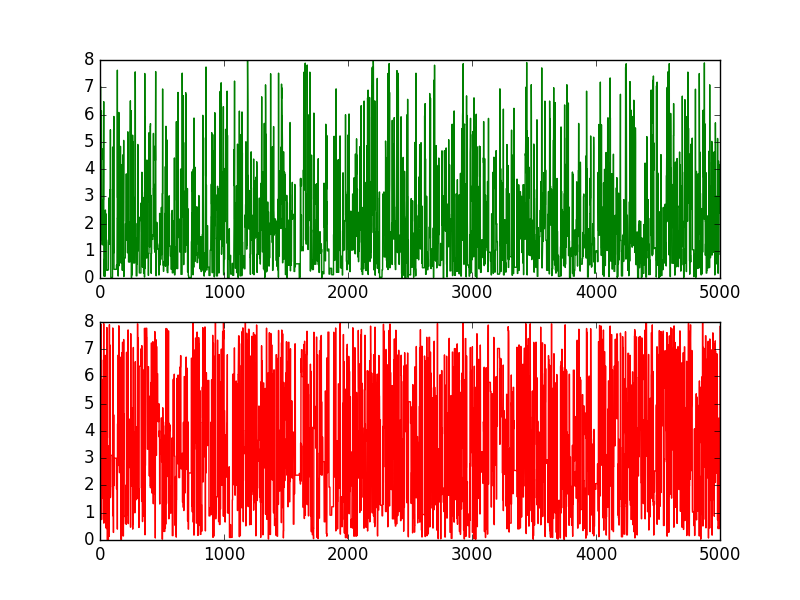
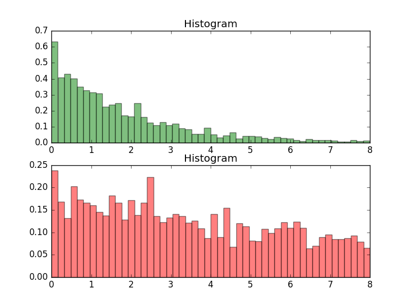
3.1、Blockwise
实验代码
'''
Date:20160703
@author: zhaozhiyong
'''
import random
import math
from scipy.stats import norm
import matplotlib.pyplot as plt
def bivexp(theta1, theta2):
lam1 = 0.5
lam2 = 0.1
lam = 0.01
maxval = 8
y = math.exp(-(lam1 + lam) * theta1 - (lam2 + lam) * theta2 - lam * maxval)
return y
T = 5000
sigma = 1
thetamin = 0
thetamax = 8
theta_1 = [0.0] * (T + 1)
theta_2 = [0.0] * (T + 1)
theta_1[0] = random.uniform(thetamin, thetamax)
theta_2[0] = random.uniform(thetamin, thetamax)
t = 0
while t < T:
t = t + 1
theta_star_0 = random.uniform(thetamin, thetamax)
theta_star_1 = random.uniform(thetamin, thetamax)
alpha = min(1, (bivexp(theta_star_0, theta_star_1) / bivexp(theta_1[t - 1], theta_2[t - 1])))
u = random.uniform(0, 1)
if u <= alpha:
theta_1[t] = theta_star_0
theta_2[t] = theta_star_1
else:
theta_1[t] = theta_1[t - 1]
theta_2[t] = theta_2[t - 1]
plt.figure(1)
ax1 = plt.subplot(211)
ax2 = plt.subplot(212)
plt.ylim(thetamin, thetamax)
plt.sca(ax1)
plt.plot(range(T + 1), theta_1, 'g-', label="0")
plt.sca(ax2)
plt.plot(range(T + 1), theta_2, 'r-', label="1")
plt.show()
plt.figure(2)
ax1 = plt.subplot(211)
ax2 = plt.subplot(212)
num_bins = 50
plt.sca(ax1)
plt.hist(theta_1, num_bins, normed=1, facecolor='green', alpha=0.5)
plt.title('Histogram')
plt.sca(ax2)
plt.hist(theta_2, num_bins, normed=1, facecolor='red', alpha=0.5)
plt.title('Histogram')
plt.show()
- 1
- 2
- 3
- 4
- 5
- 6
- 7
- 8
- 9
- 10
- 11
- 12
- 13
- 14
- 15
- 16
- 17
- 18
- 19
- 20
- 21
- 22
- 23
- 24
- 25
- 26
- 27
- 28
- 29
- 30
- 31
- 32
- 33
- 34
- 35
- 36
- 37
- 38
- 39
- 40
- 41
- 42
- 43
- 44
- 45
- 46
- 47
- 48
- 49
- 50
- 51
- 52
- 53
- 54
- 55
- 56
- 57
- 58
- 59
- 60
- 61
- 62
实验结果
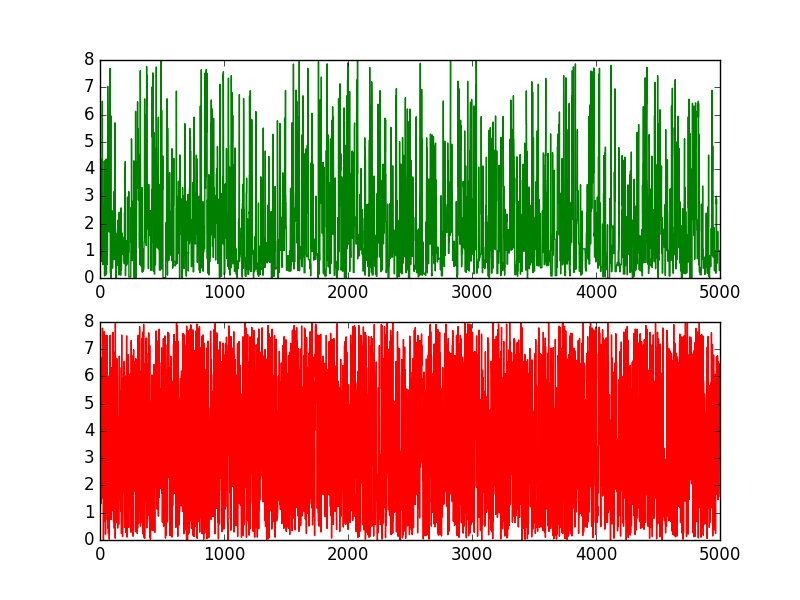
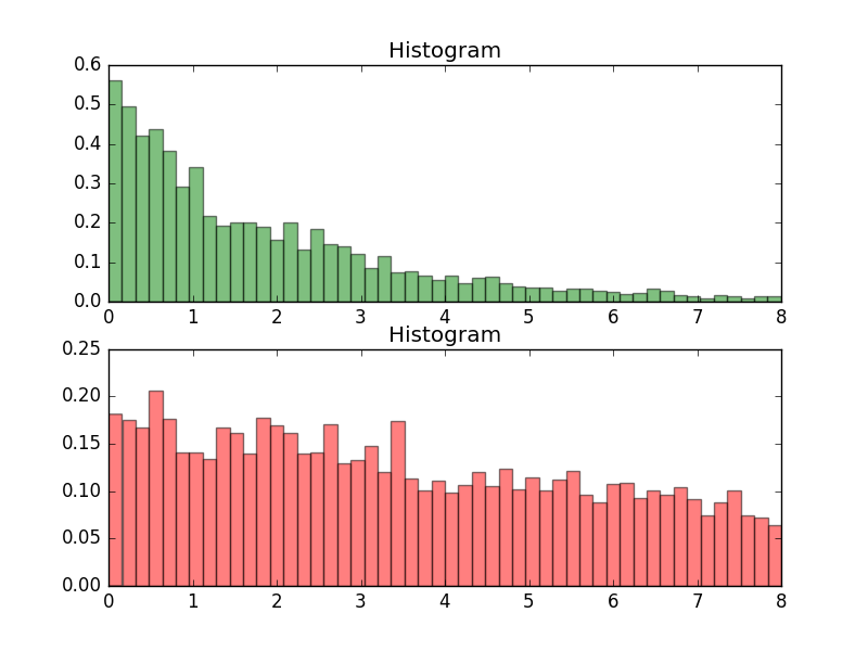
3.2、Componentwise
实验代码
'''
Date:20160703
@author: zhaozhiyong
'''
import random
import math
from scipy.stats import norm
import matplotlib.pyplot as plt
def bivexp(theta1, theta2):
lam1 = 0.5
lam2 = 0.1
lam = 0.01
maxval = 8
y = math.exp(-(lam1 + lam) * theta1 - (lam2 + lam) * theta2 - lam * maxval)
return y
T = 5000
sigma = 1
thetamin = 0
thetamax = 8
theta_1 = [0.0] * (T + 1)
theta_2 = [0.0] * (T + 1)
theta_1[0] = random.uniform(thetamin, thetamax)
theta_2[0] = random.uniform(thetamin, thetamax)
t = 0
while t < T:
t = t + 1
theta_star_1 = random.uniform(thetamin, thetamax)
alpha = min(1, (bivexp(theta_star_1, theta_2[t - 1]) / bivexp(theta_1[t - 1], theta_2[t - 1])))
u = random.uniform(0, 1)
if u <= alpha:
theta_1[t] = theta_star_1
else:
theta_1[t] = theta_1[t - 1]
theta_star_2 = random.uniform(thetamin, thetamax)
alpha = min(1, (bivexp(theta_1[t], theta_star_2) / bivexp(theta_1[t], theta_2[t - 1])))
u = random.uniform(0, 1)
if u <= alpha:
theta_2[t] = theta_star_2
else:
theta_2[t] = theta_2[t - 1]
plt.figure(1)
ax1 = plt.subplot(211)
ax2 = plt.subplot(212)
plt.ylim(thetamin, thetamax)
plt.sca(ax1)
plt.plot(range(T + 1), theta_1, 'g-', label="0")
plt.sca(ax2)
plt.plot(range(T + 1), theta_2, 'r-', label="1")
plt.show()
plt.figure(2)
ax1 = plt.subplot(211)
ax2 = plt.subplot(212)
num_bins = 50
plt.sca(ax1)
plt.hist(theta_1, num_bins, normed=1, facecolor='green', alpha=0.5)
plt.title('Histogram')
plt.sca(ax2)
plt.hist(theta_2, num_bins, normed=1, facecolor='red', alpha=0.5)
plt.title('Histogram')
plt.show()
- 1
- 2
- 3
- 4
- 5
- 6
- 7
- 8
- 9
- 10
- 11
- 12
- 13
- 14
- 15
- 16
- 17
- 18
- 19
- 20
- 21
- 22
- 23
- 24
- 25
- 26
- 27
- 28
- 29
- 30
- 31
- 32
- 33
- 34
- 35
- 36
- 37
- 38
- 39
- 40
- 41
- 42
- 43
- 44
- 45
- 46
- 47
- 48
- 49
- 50
- 51
- 52
- 53
- 54
- 55
- 56
- 57
- 58
- 59
- 60
- 61
- 62
- 63
- 64
- 65
- 66
- 67
- 68
- 69
实验结果
转自http://m.blog.csdn.net/article/details?id=51785156