Programming Exercise 7.2:Principal Component Analysis(PCA)
Python版本3.6
编译环境:anaconda Jupyter Notebook
链接:实验数据和实验指导书
提取码:i7co
本章课程笔记部分见:14.降维
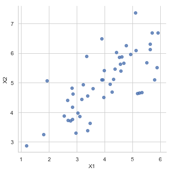
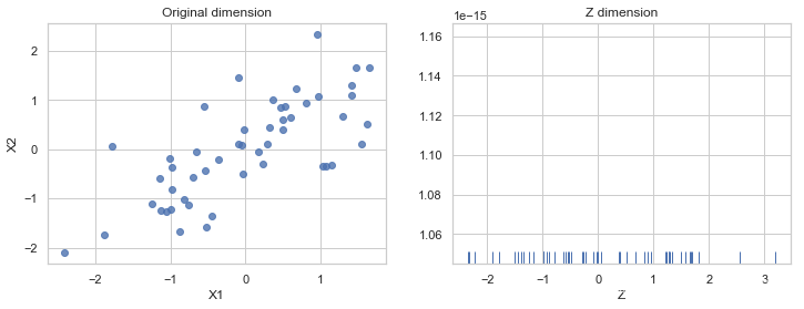
PCA是在数据集中找到“主成分”或最大方差方向的线性变换。 它可以用于降维。 在本练习中,我们首先负责实现PCA并将其应用于一个简单的二维数据集,以了解它是如何工作的。 我们从加载和可视化数据集开始。
%matplotlib inline
#IPython的内置magic函数,可以省掉plt.show(),在其他IDE中是不会支持的
import numpy as np
import pandas as pd
import matplotlib as mpl
import matplotlib.pyplot as plt
import seaborn as sns
import scipy.io as sio
sns.set(style="whitegrid",color_codes=True)
4-二维的PCA
mat = sio.loadmat('./data/ex7data1.mat')
X = mat['X']
def get_X(df):
    """
    use concat to add intersect feature to avoid side effect
    not efficient for big dataset though
    """
    ones = pd.DataFrame({'ones': np.ones(len(df))})
    data = pd.concat([ones, df], axis=1)  # column concat
    return data.iloc[:, :-1].as_matrix()  # this return ndarray, not matrix


def get_y(df):
    '''assume the last column is the target'''
    return np.array(df.iloc[:, -1])


def normalize_feature(df):
    """Applies function along input axis(default 0) of DataFrame."""
    return df.apply(lambda column: (column - column.mean()) / column.std())
sns.lmplot('X1', 'X2',
           data=pd.DataFrame(X, columns=['X1', 'X2']),
           fit_reg=False)
<seaborn.axisgrid.FacetGrid at 0x8bf2e6c9e8>
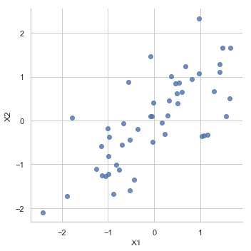
normalize data
# support functions ---------------------------------------
def plot_n_image(X, n):
    """ plot first n images
    n has to be a square number
    """
    pic_size = int(np.sqrt(X.shape[1]))
    grid_size = int(np.sqrt(n))

    first_n_images = X[:n, :]

    fig, ax_array = plt.subplots(nrows=grid_size, ncols=grid_size,
                                    sharey=True, sharex=True, figsize=(8, 8))

    for r in range(grid_size):
        for c in range(grid_size):
            ax_array[r, c].imshow(first_n_images[grid_size * r + c].reshape((pic_size, pic_size)))
            plt.xticks(np.array([]))
            plt.yticks(np.array([]))


# PCA functions ---------------------------------------
def covariance_matrix(X):
    """
    Args:
        X (ndarray) (m, n)
    Return:
        cov_mat (ndarray) (n, n):
            covariance matrix of X
    """
    m = X.shape[0]

    return (X.T @ X) / m


def normalize(X):
    """
        for each column, X-mean / std
    """
    X_copy = X.copy()
    m, n = X_copy.shape

    for col in range(n):
        X_copy[:, col] = (X_copy[:, col] - X_copy[:, col].mean()) / X_copy[:, col].std()

    return X_copy


def pca(X):
    """
    http://docs.scipy.org/doc/numpy/reference/generated/numpy.linalg.svd.html
    Args:
        X ndarray(m, n)
    Returns:
        U ndarray(n, n): principle components
    """
    # 1. normalize data
    X_norm = normalize(X)

    # 2. calculate covariance matrix
    Sigma = covariance_matrix(X_norm)  # (n, n)

    # 3. do singular value decomposition
    # remeber, we feed cov matrix in SVD, since the cov matrix is symmetry
    # left sigular vector and right singular vector is the same, which means
    # U is V, so we could use either one to do dim reduction
    U, S, V = np.linalg.svd(Sigma)  # U: principle components (n, n)

    return U, S, V


def project_data(X, U, k):
    """
    Args:
        U (ndarray) (n, n)
    Return:
        projected X (n dim) at k dim
    """
    m, n = X.shape

    if k > n:
        raise ValueError('k should be lower dimension of n')

    return X @ U[:, :k]


def recover_data(Z, U):
    m, n = Z.shape

    if n >= U.shape[0]:
        raise ValueError('Z dimension is >= U, you should recover from lower dimension to higher')

    return Z @ U[:, :n].T
X_norm = normalize(X)

sns.lmplot('X1', 'X2',
           data=pd.DataFrame(X_norm, columns=['X1', 'X2']),
           fit_reg=False)
<seaborn.axisgrid.FacetGrid at 0x8be9d90c18>
covariance matrix
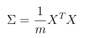
Sigma =covariance_matrix(X_norm)  # capital greek Sigma
Sigma  # (n, n)
array([[1.        , 0.73553038],
       [0.73553038, 1.        ]])
PCA
U, S, V = pca(X_norm)
project data to lower dimension
Z = project_data(X_norm, U, 1)
Z[:10]
array([[ 1.49631261],
       [-0.92218067],
       [ 1.22439232],
       [ 1.64386173],
       [ 1.2732206 ],
       [-0.97681976],
       [ 1.26881187],
       [-2.34148278],
       [-0.02999141],
       [-0.78171789]])
fig, (ax1, ax2) = plt.subplots(ncols=2, figsize=(12, 4))

sns.regplot('X1', 'X2',
           data=pd.DataFrame(X_norm, columns=['X1', 'X2']),
           fit_reg=False,
           ax=ax1)
ax1.set_title('Original dimension')

sns.rugplot(Z, ax=ax2)
ax2.set_xlabel('Z')
ax2.set_title('Z dimension')
Text(0.5, 1.0, 'Z dimension')
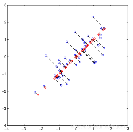
recover data to original dimension
X_recover = recover_data(Z, U)

fig, (ax1, ax2, ax3) = plt.subplots(ncols=3, figsize=(12, 4))

sns.rugplot(Z, ax=ax1)
ax1.set_title('Z dimension')
ax1.set_xlabel('Z')

sns.regplot('X1', 'X2',
           data=pd.DataFrame(X_recover, columns=['X1', 'X2']),
           fit_reg=False,
           ax=ax2)
ax2.set_title("2D projection from Z")

sns.regplot('X1', 'X2',
           data=pd.DataFrame(X_norm, columns=['X1', 'X2']),
           fit_reg=False,
           ax=ax3)
ax3.set_title('Original dimension')
Text(0.5, 1.0, 'Original dimension')

the projection from (X1, X2) to Z could be visualized like this
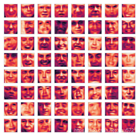
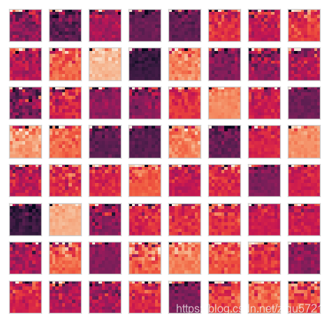
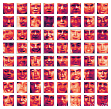
5-PCA用于面部数据
此练习中的最后一个任务是将PCA应用于脸部图像。 通过使用相同的降维技术,我们可以使用比原始图像少得多的数据来捕获图像的“本质”。
mat = sio.loadmat('./data/ex7faces.mat')
mat.keys()
dict_keys(['__header__', '__version__', '__globals__', 'X'])
X = np.array([x.reshape((32, 32)).T.reshape(1024) for x in mat.get('X')])
X.shape
(5000, 1024)
# support functions ---------------------------------------
def plot_n_image(X, n):
    """ plot first n images
    n has to be a square number
    """
    pic_size = int(np.sqrt(X.shape[1]))
    grid_size = int(np.sqrt(n))

    first_n_images = X[:n, :]

    fig, ax_array = plt.subplots(nrows=grid_size, ncols=grid_size,
                                    sharey=True, sharex=True, figsize=(8, 8))

    for r in range(grid_size):
        for c in range(grid_size):
            ax_array[r, c].imshow(first_n_images[grid_size * r + c].reshape((pic_size, pic_size)))
            plt.xticks(np.array([]))
            plt.yticks(np.array([]))


# PCA functions ---------------------------------------
def covariance_matrix(X):
    """
    Args:
        X (ndarray) (m, n)
    Return:
        cov_mat (ndarray) (n, n):
            covariance matrix of X
    """
    m = X.shape[0]

    return (X.T @ X) / m


def normalize(X):
    """
        for each column, X-mean / std
    """
    X_copy = X.copy()
    m, n = X_copy.shape

    for col in range(n):
        X_copy[:, col] = (X_copy[:, col] - X_copy[:, col].mean()) / X_copy[:, col].std()

    return X_copy


def pca(X):
    """
    http://docs.scipy.org/doc/numpy/reference/generated/numpy.linalg.svd.html
    Args:
        X ndarray(m, n)
    Returns:
        U ndarray(n, n): principle components
    """
    # 1. normalize data
    X_norm = normalize(X)

    # 2. calculate covariance matrix
    Sigma = covariance_matrix(X_norm)  # (n, n)

    # 3. do singular value decomposition
    # remeber, we feed cov matrix in SVD, since the cov matrix is symmetry
    # left sigular vector and right singular vector is the same, which means
    # U is V, so we could use either one to do dim reduction
    U, S, V = np.linalg.svd(Sigma)  # U: principle components (n, n)

    return U, S, V


def project_data(X, U, k):
    """
    Args:
        U (ndarray) (n, n)
    Return:
        projected X (n dim) at k dim
    """
    m, n = X.shape

    if k > n:
        raise ValueError('k should be lower dimension of n')

    return X @ U[:, :k]


def recover_data(Z, U):
    m, n = Z.shape

    if n >= U.shape[0]:
        raise ValueError('Z dimension is >= U, you should recover from lower dimension to higher')

    return Z @ U[:, :n].T
plot_n_image(X, n=64)

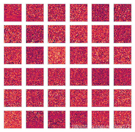
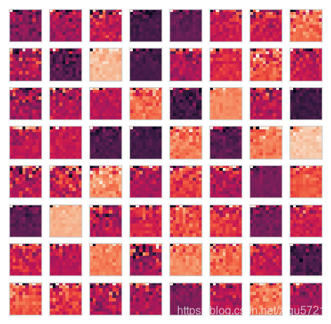
run PCA, find principle components
U, _, _ = pca(X)
U.shape
(1024, 1024)
plot_n_image(U, n=36)
reduce dimension to k=100
Z = project_data(X, U, k=100)
plot_n_image(Z, n=64)
recover from k=100
X_recover = recover_data(Z, U)
plot_n_image(X_recover, n=64)
sklearn PCA
from sklearn.decomposition import PCA
sk_pca = PCA(n_components=100)
Z = sk_pca.fit_transform(X)
Z.shape
(5000, 100)
plot_n_image(Z, 64)
X_recover = sk_pca.inverse_transform(Z)
X_recover.shape
(5000, 1024)
plot_n_image(X_recover, n=64)