第3次作业:Mini Batch 梯度下降
| 项目 |
内容
|
|---|---|
| 这个作业属于哪个课程 | |
| 这个作业的要求在哪里 | |
| 我在这个课程的目标是 |
学会、理解和应用神经网络知识来完成一个app
|
| 这个作业在哪个具体方面帮助我实现目标 |
学会小批量梯度下降的原理和实际代码实现
|
| 作业正文 | |
| 参考文献 |
一、作业要求
- 采用随机选取数据的方式
- batch size分别选择5,10,15进行运行
二、代码
import numpy as np
import matplotlib.pyplot as plt
from pathlib import Path

class CData(object):
    def __init__(self, loss, w, b, epoch, iteration):
        self.loss = loss
        self.w = w
        self.b = b
        self.epoch = epoch
        self.iteration = iteration

def ReadData():
    Xfile = Path("D:\Python\TemperatureControlXData.dat")
    Yfile = Path("D:\Python\TemperatureControlYData.dat")
    if Xfile.exists() & Yfile.exists():
        X = np.load(Xfile)
        Y = np.load(Yfile)
        return X.reshape(1,-1), Y.reshape(1,-1)
    else:
        return None,None

def ForwardCalculationBatch(W, B, batch_x):
    Z = np.dot(W, batch_x) + B
    return Z

def BackPropagationBatch(batch_x, batch_y, batch_z):
    m = batch_x.shape[1]
    dZ = batch_z - batch_y
    dB = dZ.sum(axis=1, keepdims = True)/m
    dW = np.dot(dZ, batch_x.T)/m
    return dW, dB

def UpdateWeights(w, b, dW, dB, eta):
    w = w - eta*dW
    b = b - eta*dB
    return w,b

def CheckLoss(W, B, X, Y):
    m = X.shape[1]
    Z = np.dot(W, X) + B
    LOSS = (Z -Y)**2 #MSE
    loss = LOSS.sum()/m/2
    return loss

def Shuffle(X,Y,num_feature):
    seq = np.arange(0,num_feature)
    # Shuffle the X and Y arrays
    np.random.shuffle(seq)
    X = np.array(X[seq])
    Y = np.array(Y[seq])
    return X, Y

def GetBatchSample(X, Y, batch_size, iteration,num_feature):
    start = iteration * batch_size
    end = start + batch_size
    batch_x = X[0:num_feature,start:end].reshape(num_feature,batch_size)
    batch_y = Y[0,start:end].reshape(1,batch_size)
    return batch_x, batch_y

if __name__ == "__main__":
    # MiniBatch Method
    learning_rate = [0.01,0.1,0.5] #eta
    max_epoch = 50
    batch_size_sample = [5,10,15]
    color = ['orange','red','green']

    for eta in learning_rate:
        i = 0
        for batch_size in batch_size_sample:
            X, Y = ReadData()
            W = np.zeros((1, 1))
            B = np.zeros((1,1))

            # calculate loss to decide the stop condition
            loss = 5
            dict_loss = {}
            # count of samples
            num_example = X.shape[1]
            num_feature = X.shape[0]
            max_iteration = (int)(num_example/batch_size)
            X, Y = Shuffle(X,Y,num_feature)

            for epoch in range (max_epoch):
                print("epoch = %d" %epoch)
                for iteration in range(max_iteration):
                    batch_x, batch_y = GetBatchSample(X,Y,batch_size,iteration,num_feature)
                    batch_z = ForwardCalculationBatch(W, B, batch_x)
                    dW, dB = BackPropagationBatch(batch_x, batch_y, batch_z)# calculate gradient of w and b
                    W, B = UpdateWeights(W, B, dW, dB, eta)# update w,b
                    loss = CheckLoss(W,B,X,Y)#calculate loss
                    prev_loss = loss
                    dict_loss[loss] = CData(loss,W,B,epoch,iteration)

            loss = []
            for key in dict_loss:
                loss.append(key)

            plt.plot(loss[30:800], color = color[i], label = 'batch_size ='+str(batch_size))
            i = i+1

        plt.title("Mini Batch, Learning Rate at "+str(eta))
        plt.xlabel("epoch")
        plt.ylabel("loss")
        plt.legend(loc='upper right')
        plt.show()
运行结果:
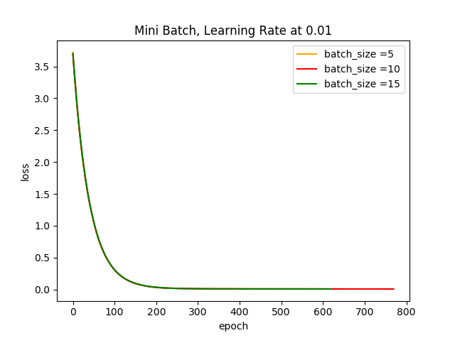
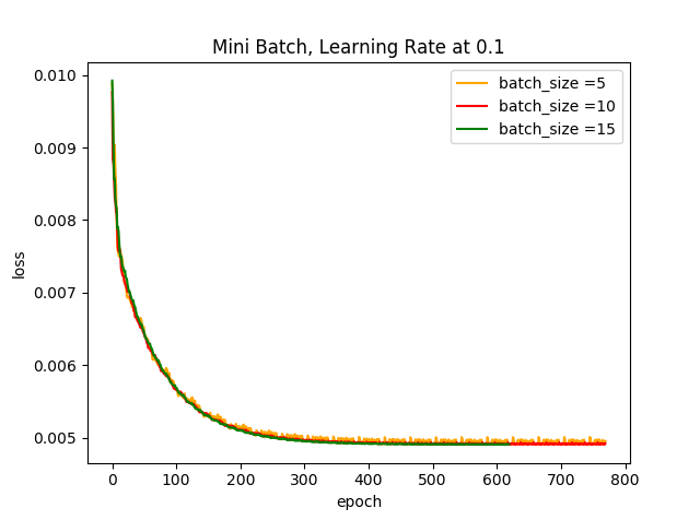
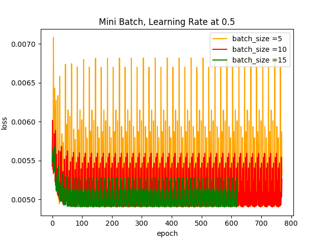
结果分析:
根据以上两个图可知,学习步长越小,Loss曲线的光滑程度会越大,若此时的学习步长为0.01,基本上可以忽略数据集小批量的大小;当学习步长较大时,可以很明显的看出batch size越小对其Loss曲线产生的的波动程度越大,这是因为受几个样本(小批量)的影响最大,到后期徘徊不前,在最优解附近震荡。
三、问题解答
问题二:为什么是椭圆而不是圆?如何把这个图变成一个圆?
Ans: 椭圆的一般表达式为\(Ax^2+By^2+Cxy+Dx+eY = 1\)
而损失函数,$ Loss =\frac{1}{2m}\displaystyle\sum_{i=1}^{m} (y_i - wx_i - b)^2 $
\(=\displaystyle\sum_{i=1}^{m} (w^2x_i^2 + b^2 + 2x_ibw-2y_ib-2x_iy_iw+y_i^2)\)
可见损失函数为一椭圆函数。
圆的一般表达式为:
$(x-h)^2+(y-k)^2 = r^2 $
$ x^2+y^2-2hx-2ky+(y^2+k^2-r^2)=0$
当损失函数中的\(2x_ibw-2y\)的系数为零时,且\(w^2,b^2\)同时大于零,损失函数就是一圆方程。
问题三:为什么中心是个椭圆区域而不是一个点?
Ans: Loss函数中计算了一系列离散的数据点,并将计算出的一系列损失函数值存放在矩阵中,并把一系列相近的损失函数值连成线形成椭圆。损失函数图的中心不会是一个点,因为不是所有的数据点都在损失函数曲线上,损失函数没办法计算出一个真实的全局最优解。若要在中心产生一个点,损失函数需为单峰函数,中心点为该函数的极小值点,也是全局最优解。