【R描述统计分析】绘图命令
高水平绘图函数
高水平作图函数: plot( ) 、pairs( ) 、coplot( )、qqnorm( ) 、qqline( ) 、hist( )、contour( )
plot()函数
一般意义:
plot(x) 针对一列数
plot(x,y) 针对两列数
x<-rnorm(100,0,1)
y<-x+rnorm(100,0,1)
plot(x)
plot(x,y)

应用:

y<-c(1600, 1610, 1650, 1680, 1700, 1700, 1780, 1500, 1640,
     1400, 1700, 1750, 1640, 1550, 1600, 1620, 1640, 1600,
     1740, 1800, 1510, 1520, 1530, 1570, 1640, 1600)
f<-factor(c(rep(1,7),rep(2,5), rep(3,8), rep(4,6)))
plot(f,y)

显示多变量数据
df<-data.frame(
  Age=c(13, 13, 14, 12, 12, 15, 11, 15, 14, 14, 14, 15,
        12, 13, 12, 16, 12, 11, 15 ),
  Height=c(56.5, 65.3, 64.3, 56.3, 59.8, 66.5, 51.3,
           62.5, 62.8, 69.0, 63.5, 67.0, 57.3, 62.5,
           59.0, 72.0, 64.8, 57.5, 66.5),
  Weight=c( 84.0,  98.0,  90.0,  77.0,  84.5, 112.0,
            50.5, 112.5, 102.5, 112.5, 102.5, 133.0,
            83.0,  84.0,  99.5, 150.0, 128.0,  85.0,
           112.0)
)
plot(df)
attach(df)
plot(~Age+Height)
plot(Weight~Age+Height)

pairs(df)
coplot(Weight ~ Height | Age)
显示图形


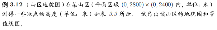
实例1:山区地貌图

x<-seq(0,2800, 400); y<-seq(0,2400,400)
z<-scan()
1180 1320 1450 1420 1400 1300  700  900
1230 1390 1500 1500 1400  900 1100 1060
1270 1500 1200 1100 1350 1450 1200 1150
1370 1500 1200 1100 1550 1600 1550 1380
1460 1500 1550 1600 1550 1600 1600 1600
1450 1480 1500 1550 1510 1430 1300 1200
1430 1450 1470 1320 1280 1200 1080  940

Z<-matrix(z, nrow=8)
image(x, y, Z)
contour(x, y, Z, levels = seq(min(z), max(z), by = 80))
persp(x, y, Z)

得到一幅等值线图:

和一幅三维图:

实例2:绘制等值线图和三维曲面图

x<-y<-seq(-2*pi, 2*pi, pi/15)
f<-function(x,y) sin(x)*sin(y)
z<-outer(x,y, f)
contour(x,y,z,col="blue")
persp(x,y,z,theta=30, phi=30, expand=0.7,col="lightblue")
得到图像:


低水平作图函数
加点与线的函数
加点函数 points()
加线函数 lines()
在点处加标记
test()
在图上加直线
abline(a,b): 画一条y=a+bx
abline(h=y) :过所有点的水平直线
abline(v=x):过所有点的竖直直线
abline(lm.obj):绘出线性模型得出的线性方程
