import pandas as pd
import numpy as np
import matplotlib.pyplot as plt
import matplotlib.style as style
import seaborn as sns
import warnings

warnings.filterwarnings('ignore')

style.use('fivethirtyeight')
plt.rcParams['figure.figsize']=(8,4)
plt.rcParams['font.family']=['SimHei']
plt.rcParams['axes.unicode_minus']=False

bj=pd.read_csv('./beijing.csv')
bj.info()
结果:数据的基本信息
<class 'pandas.core.frame.DataFrame'>
Int64Index: 16210 entries, 0 to 16209
Data columns (total 8 columns):
城区        16210 non-null object
卧室数       16210 non-null int64
客厅数       16210 non-null int64
房屋面积      16210 non-null float64
楼层        16210 non-null object
是否临近地铁    16210 non-null int64
是否学区房     16210 non-null int64
单位面积价格    16210 non-null int64
dtypes: float64(1), int64(5), object(2)
memory usage: 1.1+ MB
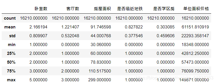
bj.describe()
结果:
bj.groupby('城区').城区.count()
结果:
城区
东城     2783
丰台     2947
朝阳     2864
海淀     2919
石景山    1947
西城     2750
Name: 城区, dtype: int64
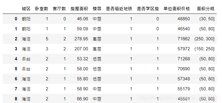
离散化和分箱
bins=[30,50,80,100,120,150,250,300]
bj['面积分组']=pd.cut(bj.房屋面积,bins)
bj
结果:
bj.groupby('面积分组').面积分组.count()
结果:
面积分组
(30, 50]      1422
(50, 80]      6890
(80, 100]     2896
(100, 120]    1614
(120, 150]    1729
(150, 250]    1501
(250, 300]     158
Name: 面积分组, dtype: int64
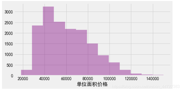
价格分布
sns.distplot(a=bj.单位面积价格,kde=False,color='purple',bins=13)
结果:
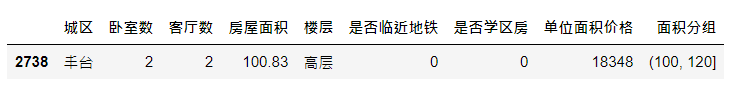
min_price=bj.单位面积价格.min()
bj.query(f"单位面积价格=={min_price}")
结果:
max_price=bj.单位面积价格.max()
bj.query(f"单位面积价格=={max_price}")
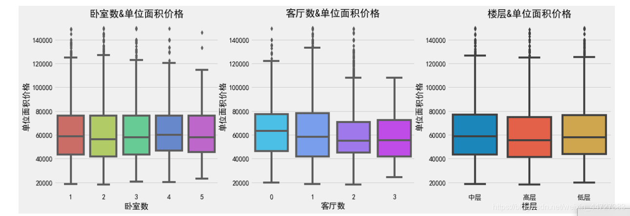
描述性分析
fig,(ax1,ax2,ax3)=plt.subplots(nrows=1,ncols=3,figsize=(3*6,6))
sns.boxplot(x='卧室数', y='单位面积价格', data=bj,ax = ax1,palette='hls')
ax1.set_title('卧室数&单位面积价格')
sns.boxplot(x='客厅数',y='单位面积价格',data=bj,ax=ax2,palette='cool')
ax2.set_title('客厅数&单位面积价格')
sns.boxplot(x='楼层', y='单位面积价格', data=bj,ax = ax3)
ax3.set_title('楼层&单位面积价格')
结果:
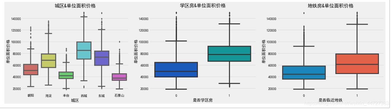
fig,(ax1,ax2,ax3) = plt.subplots(nrows=1,ncols=3,figsize=(4*6,6))

sns.boxplot(x='城区', y='单位面积价格', data=bj,ax = ax1,palette='hls')
ax1.set_title('城区&单位面积价格')
sns.boxplot(x='是否学区房', y='单位面积价格', data=bj,ax = ax2,palette='winter')
ax2.set_title('学区房&单位面积价格')
sns.boxplot(x='是否临近地铁', y='单位面积价格', data=bj,ax = ax3)
ax3.set_title('地铁房&单位面积价格')
结果:
预测单位面积价格
- 所有的特征都是"类别型",线性回归无解,所以要用交叉项的回归
from sklearn.model_selection import train_test_split
from sklearn.linear_model import SGDRegressor,ElasticNet,LinearRegression
from sklearn.preprocessing import StandardScaler
features=bj.loc[:,['城区','是否临近地铁','是否学区房']]
labels=bj.loc[:,['单位面积价格']]
features['城区']=features['城区'].astype('category').cat.codes
from sklearn.externals.six import StringIO
import sklearn.tree as tree
import pydotplus

from sklearn.tree import DecisionTreeRegressor

cartReg=DecisionTreeRegressor().fit(features,labels)

cartReg.score(features,labels)
 >> 0.5980859207408644
X_test = [[2,1,1]]
price = cartReg.predict(X_test)
print(price,90*price)
>> [57713.91947566] [5194252.75280899]
调用画图工具,要先安装graphviz ,并将其添加到环境变量中
str_ = StringIO() #保存模型的输出 brew install graphviz
'''
decision_tree : 决策树实例对象
out_file :制定输出的位置
feature_names : 特征的名称
filled :填充颜色
rounded :圆角化
'''
tree.export_graphviz(cartReg,str_,feature_names=['District','Subway','School'],filled=True,rounded=True)

graph = pydotplus.graph_from_dot_data(str_.getvalue())

graph.write_jpg('cartReg.jpg')
