目录
【若觉文章质量良好且有用,请别忘了点赞收藏加关注,这将是我继续分享的动力,万分感谢!】
其他:
1.时间序列转二维图像方法及其应用研究综述_vm-1215的博客-CSDN博客
2.将时间序列转成图像——小波变换方法 Matlab实现_vm-1215的博客-CSDN博客
3.将时间序列转成图像——希尔伯特-黄变换方法 Matlab实现_vm-1215的博客-CSDN博客
1 方法
短时傅里叶变换(Short Time Fourier Transform, STFT)是傅里叶变换(Fourier Transform, FT)的一种变形,以确认时变信号的频率和相位在时间轴上的变化情况。其基本思想是:选择一个合适的窗函数(常见有方形、三角形、高斯函数等),假设时变信号在这个短时间间隔的窗内是一个平稳的信号,通过傅里叶变换计算出信号的频率和相位信息,然后在时间轴上移动窗函数,计算出不同短时间段内信号的频率和相位,最终实现信号的时频分析,得到其对应的时频图。
其中, 为时间窗函数。 根据短时傅里叶变化的定义,给定时变信号
, 其编码步骤如下:
- 确定参数:信号长度
, 采样频率
, 窗口长度
, 步长
, 窗函数,重叠点数
;
- 计算窗口滑定初始滑动次数为
, 构造一个大小为
、元素值都为0的初始时频矩阵
。
- 根据当前窗口位蝠,截取信号片段,进行快速傅里叶变换,得到当前窗口中信号片段所对应的频率分布, 记为列向量
;
- 更新当前滑动次数 :
, 更新时频矩阵
;
- 判断当前滑动次数
是否等于总滑动次数
, 若是 : 编码完成, 输出时频矩阵
短时傅里叶变换的实现流程简单, 处理时间短且应用广泛, 但其时频分析后的时间-频 率窗口大小不变, 很难捕捉到一些细小的局部信息。
2 Matlab代码实现
clear, close all
%% initialize parameters
samplerate = 500; % in Hz
nfft = 64; % try to use 32 or 16 to investigate the trade off between time and frequency resolution
noverlap = round(nfft*0.5); % number of overlapping points (50%)
%% generate simulated signals with step changes in frequency
data = csvread('3_1_link6_28_5_30min.csv'); % input the signal from the Excle
data = data'; % change the signal from column to row
N = length(data); % calculate the length of the data
taxis = [1:N]/samplerate; % time axis for whole data length
figure, % plot the origianl signal
plot(taxis,data),xlim([taxis(1) taxis(end)])
xlabel('Time (s)')
%% calculate spectrogram using STFT
[spec,faxis,taxis]=spectrogram(data,hamming(nfft),noverlap,nfft,samplerate);
Mag=abs(spec); % get spectrum magnitude
im = figure;
imagesc(taxis,faxis,Mag) % plot spectrogram as 2D imagsc
colorbar
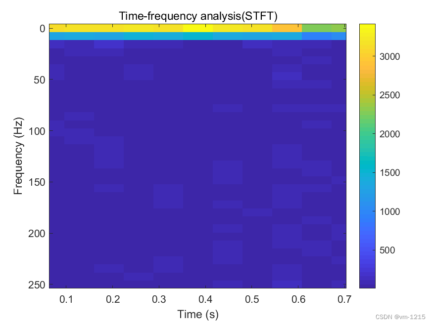
title('Time-frequency analysis(STFT)')
xlabel('Time (s)'),xlim([taxis(1) taxis(end)])
ylabel('Frequency (Hz)')
saveas(im,'STFT_1.bmp')3 结果
【若觉文章质量良好且有用,请别忘了点赞收藏加关注,这将是我继续分享的动力,万分感谢!】