说明

半图解法计算步骤如下:
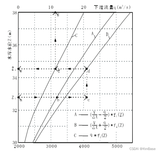
(1)根据水位～库容关系、水位～泄流关系以及计算时段等绘制辅助曲线；
(2)确定起调水位$Z_1$及相应的$q_1$、$V_1$计算各时段平均入库流量$Q_p$；
(3)在水位坐标轴上确定Z位置,记为a点。作水平线ac 交A线于b点,使$bc=Q_p$。因A 线为$(V/\Delta t-q/2)=f_1(Z)$,则$ab$等于$(V/\Delta t-q/2)$，$ac$等于$Q,+(V\Delta t-q/2)=(V/\Delta t+q/2)$。
(4)在c点做垂线交B线于d点,由d点作水平线de 交Z坐标轴于e点，可见$de=ac=(V/\Delta t+q/2)$。因B线为$(V/At+q/2)=f(Z)$，$d$ 点位于$B$线上,则$e$点为$Z$值。
(5)过$de$与$C$线交点f作垂线交$q$坐标轴于$g$点,则$g$点为$q$值。
(6)根据水量平衡得到下一时刻的$V$。
(7)将$e$点的$Z$值作为第二时段的$Z$,重复(2)~(6)即可得下一时段的特征值。由此逐时段进行计算,即可完成全部计算。

Python代码

def half_figure():
    z, v, q = util.ZVQ[:, 0], util.ZVQ[:, 1], util.ZVQ[:, 2]
    y = v*10**8/util.DT+q/2
    # 散点图
    plt.scatter(y, q, label='scatter')
    # 插值
    fyq = interpolate.interp1d(y, q, 'quadratic')
    ynew = np.linspace(min(y), max(y), len(y)*100)
    qnew = fyq(ynew)
    plt.plot(ynew, qnew, 'g--', label='interpolate')
    # 拟合
    z1 = np.polyfit(y, q, 3)
    p1 = np.poly1d(z1)
    plt.plot(y, p1(y), 'r-', label='polyfit')
    # 调整图像
    plt.xlabel("$\\frac{V}{\\Delta t}+\\frac{q}{2}(m^3/s)$")
    plt.ylabel("$q(m^3/s)$")
    plt.title("$q-\\frac{V}{\\Delta t}+\\frac{q}{2}$")
    plt.legend()
    plt.grid()
    plt.show()

    # 计算，采用拟合图像
    q_rk = util.QIN
    T = q_rk.size
    (q_qs, q_ck, V, Z) = (0,  # 起始流量
                          np.zeros(T + 1),  # 出库流量
                          np.zeros(T + 1),  # 水库蓄水过程
                          np.zeros(T + 1))  # 水位过程
    Z[0] = util.Z_fx
    V[0] = util.fzv(Z[0])
    for t in range(0, T - 1):
        # print("<DEBUG> time [{}]".format(t))
        Q_T = util.fzq(Z[t])  # 最大过流能力
        q_ck[t] = q_qs + Q_T  # 出库流量过程
        y2 = np.average([q_rk[t], q_rk[t+1]]) - q_ck[t] + V[t] / util.DT + q_ck[t] / 2  # 计算右侧
        q2 = p1(y2)  # 查q2
        q_ck[t+1] = q2  # 放进结果
        V[t+1] = V[t] + ((q_rk[t] + q_rk[t+1]) * util.DT / 2 - (q_ck[t] + q_ck[t+1]) * util.DT / 2)/10**8  # 水量平衡
        Z[t+1] = util.fvz(V[t+1])  # 水位变化
        print(V[t])
    # 画水位变化
    plt.plot(Z[:-1])
    plt.title("$Z$")
    plt.xlabel("$T$")
    plt.ylabel("$Z(m)$")
    zmax = (np.where(Z == np.max(Z))[0][0], np.max(Z).round(1))
    plt.annotate("max{}".format(zmax), xy=zmax)
    plt.xlim(0)
    plt.grid()
    plt.show()
    # 画库容变化
    # plt.plot(V[:-1])
    # plt.title("$V$")
    # plt.xlabel("$T$")
    # plt.ylabel("$V(10^8m^3)$")
    # plt.grid()
    # plt.show()
    # 画入流出流过程线
    plt.plot(q_rk, '.-', label='In')
    inmax = (np.where(q_rk == np.max(q_rk))[0][0], np.max(q_rk))
    plt.plot(q_ck[:-2], 'r--', label='Out')
    omax = (np.where(q_ck == np.max(q_ck))[0][0], np.max(q_ck).round(1))
    plt.title("$In\\quad and\\quad Out(half-figure)$")
    plt.xlabel("$T(\\Delta T=1h)$")
    plt.ylabel("$Q(m^3/s)$")
    plt.annotate("max{}".format(inmax), xy=inmax)
    plt.annotate("max{}".format(omax), xy=omax)
    plt.xlim(0)
    plt.legend()
    plt.grid()
    plt.show()