权重初始化的 正确选择能够有效的避免多层神经网络传播过程中的梯度消失和梯度爆炸问题,下面通过三个初始化的方法来验证:
首先看数据集,init_utils.py代码,激活函数,数据集等等,代码如下:
import numpy as np
import matplotlib.pyplot as plt
import h5py
import sklearn
import sklearn.datasets

def sigmoid(x):
    """
    Compute the sigmoid of x

    Arguments:
    x -- A scalar or numpy array of any size.

    Return:
    s -- sigmoid(x)
    """
    s = 1/(1+np.exp(-x))
    return s

def relu(x):
    """
    Compute the relu of x

    Arguments:
    x -- A scalar or numpy array of any size.

    Return:
    s -- relu(x)
    """
    s = np.maximum(0,x)

    return s

def forward_propagation(X, parameters):
    """
    Implements the forward propagation (and computes the loss) presented in Figure 2.

    Arguments:
    X -- input dataset, of shape (input size, number of examples)
    Y -- true "label" vector (containing 0 if cat, 1 if non-cat)
    parameters -- python dictionary containing your parameters "W1", "b1", "W2", "b2", "W3", "b3":
                    W1 -- weight matrix of shape ()
                    b1 -- bias vector of shape ()
                    W2 -- weight matrix of shape ()
                    b2 -- bias vector of shape ()
                    W3 -- weight matrix of shape ()
                    b3 -- bias vector of shape ()

    Returns:
    loss -- the loss function (vanilla logistic loss)
    """

    # retrieve parameters
    W1 = parameters["W1"]
    b1 = parameters["b1"]
    W2 = parameters["W2"]
    b2 = parameters["b2"]
    W3 = parameters["W3"]
    b3 = parameters["b3"]

    # LINEAR -> RELU -> LINEAR -> RELU -> LINEAR -> SIGMOID
    z1 = np.dot(W1, X) + b1
    a1 = relu(z1)
    z2 = np.dot(W2, a1) + b2
    a2 = relu(z2)
    z3 = np.dot(W3, a2) + b3
    a3 = sigmoid(z3)

    cache = (z1, a1, W1, b1, z2, a2, W2, b2, z3, a3, W3, b3)

    return a3, cache

def backward_propagation(X, Y, cache):
    """
    Implement the backward propagation presented in figure 2.

    Arguments:
    X -- input dataset, of shape (input size, number of examples)
    Y -- true "label" vector (containing 0 if cat, 1 if non-cat)
    cache -- cache output from forward_propagation()

    Returns:
    gradients -- A dictionary with the gradients with respect to each parameter, activation and pre-activation variables
    """
    m = X.shape[1]
    (z1, a1, W1, b1, z2, a2, W2, b2, z3, a3, W3, b3) = cache

    dz3 = 1./m * (a3 - Y)
    dW3 = np.dot(dz3, a2.T)
    db3 = np.sum(dz3, axis=1, keepdims = True)

    da2 = np.dot(W3.T, dz3)
    dz2 = np.multiply(da2, np.int64(a2 > 0))
    dW2 = np.dot(dz2, a1.T)
    db2 = np.sum(dz2, axis=1, keepdims = True)

    da1 = np.dot(W2.T, dz2)
    dz1 = np.multiply(da1, np.int64(a1 > 0))
    dW1 = np.dot(dz1, X.T)
    db1 = np.sum(dz1, axis=1, keepdims = True)

    gradients = {"dz3": dz3, "dW3": dW3, "db3": db3,
                 "da2": da2, "dz2": dz2, "dW2": dW2, "db2": db2,
                 "da1": da1, "dz1": dz1, "dW1": dW1, "db1": db1}

    return gradients

def update_parameters(parameters, grads, learning_rate):
    """
    Update parameters using gradient descent

    Arguments:
    parameters -- python dictionary containing your parameters
    grads -- python dictionary containing your gradients, output of n_model_backward

    Returns:
    parameters -- python dictionary containing your updated parameters
                  parameters['W' + str(i)] = ...
                  parameters['b' + str(i)] = ...
    """

    L = len(parameters) // 2 # number of layers in the neural networks

    # Update rule for each parameter
    for k in range(L):
        parameters["W" + str(k+1)] = parameters["W" + str(k+1)] - learning_rate * grads["dW" + str(k+1)]
        parameters["b" + str(k+1)] = parameters["b" + str(k+1)] - learning_rate * grads["db" + str(k+1)]

    return parameters

def compute_loss(a3, Y):

    """
    Implement the loss function

    Arguments:
    a3 -- post-activation, output of forward propagation
    Y -- "true" labels vector, same shape as a3

    Returns:
    loss - value of the loss function
    """

    m = Y.shape[1]
    logprobs = np.multiply(-np.log(a3),Y) + np.multiply(-np.log(1 - a3), 1 - Y)
    loss = 1./m * np.nansum(logprobs)

    return loss

def load_cat_dataset():
    train_dataset = h5py.File('datasets/train_catvnoncat.h5', "r")
    train_set_x_orig = np.array(train_dataset["train_set_x"][:]) # your train set features
    train_set_y_orig = np.array(train_dataset["train_set_y"][:]) # your train set labels

    test_dataset = h5py.File('datasets/test_catvnoncat.h5', "r")
    test_set_x_orig = np.array(test_dataset["test_set_x"][:]) # your test set features
    test_set_y_orig = np.array(test_dataset["test_set_y"][:]) # your test set labels

    classes = np.array(test_dataset["list_classes"][:]) # the list of classes

    train_set_y = train_set_y_orig.reshape((1, train_set_y_orig.shape[0]))
    test_set_y = test_set_y_orig.reshape((1, test_set_y_orig.shape[0]))

    train_set_x_orig = train_set_x_orig.reshape(train_set_x_orig.shape[0], -1).T
    test_set_x_orig = test_set_x_orig.reshape(test_set_x_orig.shape[0], -1).T

    train_set_x = train_set_x_orig/255
    test_set_x = test_set_x_orig/255

    return train_set_x, train_set_y, test_set_x, test_set_y, classes


def predict(X, y, parameters):
    """
    This function is used to predict the results of a  n-layer neural network.

    Arguments:
    X -- data set of examples you would like to label
    parameters -- parameters of the trained model

    Returns:
    p -- predictions for the given dataset X
    """

    m = X.shape[1]
    p = np.zeros((1,m), dtype = np.int)

    # Forward propagation
    a3, caches = forward_propagation(X, parameters)

    # convert probas to 0/1 predictions
    for i in range(0, a3.shape[1]):
        if a3[0,i] > 0.5:
            p[0,i] = 1
        else:
            p[0,i] = 0

    # print results
    print("Accuracy: "  + str(np.mean((p[0,:] == y[0,:]))))

    return p

def plot_decision_boundary(model, X, y):
    # Set min and max values and give it some padding
    x_min, x_max = X[0, :].min() - 1, X[0, :].max() + 1
    y_min, y_max = X[1, :].min() - 1, X[1, :].max() + 1
    h = 0.01
    # Generate a grid of points with distance h between them
    xx, yy = np.meshgrid(np.arange(x_min, x_max, h), np.arange(y_min, y_max, h))
    # Predict the function value for the whole grid
    Z = model(np.c_[xx.ravel(), yy.ravel()])
    Z = Z.reshape(xx.shape)
    # Plot the contour and training examples
    plt.contourf(xx, yy, Z, cmap=plt.cm.Spectral)
    plt.ylabel('x2')
    plt.xlabel('x1')
    plt.scatter(X[0, :], X[1, :], c=y, cmap=plt.cm.Spectral)
    plt.show()

def predict_dec(parameters, X):
    """
    Used for plotting decision boundary.

    Arguments:
    parameters -- python dictionary containing your parameters
    X -- input data of size (m, K)

    Returns
    predictions -- vector of predictions of our model (red: 0 / blue: 1)
    """

    # Predict using forward propagation and a classification threshold of 0.5
    a3, cache = forward_propagation(X, parameters)
    predictions = (a3>0.5)
    return predictions

def load_dataset():
    np.random.seed(1)
    train_X, train_Y = sklearn.datasets.make_circles(n_samples=300, noise=.05)
    #print(train_X.shape)(300,2)
    #print(train_Y) (300,)
    np.random.seed(2)
    test_X, test_Y = sklearn.datasets.make_circles(n_samples=100, noise=.05)
    # Visualize the data  cmap = plt.cm.Spectral  表示给 1 0点不同的颜色
    plt.scatter(train_X[:, 0], train_X[:, 1], c=train_Y, s=40, cmap=plt.cm.Spectral)
    train_X = train_X.T  #(2,300)
    #print(train_X)
    train_Y = train_Y.reshape((1, train_Y.shape[0]))  #(1,300)
    #print(train_Y)
    test_X = test_X.T #(2,100)
    test_Y = test_Y.reshape((1, test_Y.shape[0]))  #(1,100)
    return train_X, train_Y, test_X, test_Y
载入数据集:
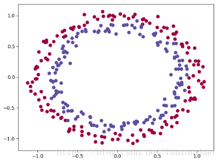
import numpy as np
import init_utils
import matplotlib.pyplot as plt
import sklearn
import sklearn.datasets
#(2, 300)(1, 300)(2, 100)(1, 100)
train_X, train_Y, test_X, test_Y=init_utils.load_dataset()
print(train_X.shape)
print(train_Y.shape)
print(test_X.shape)
print(test_Y.shape)
plt.show()
打印结果:

完整代码:
import numpy as np
import init_utils
import matplotlib.pyplot as plt
import sklearn
import sklearn.datasets
#(2, 300)(1, 300)(2, 100)(1, 100)
train_X, train_Y, test_X, test_Y=init_utils.load_dataset()
# print(train_X.shape)
# print(train_Y.shape)
# print(test_X.shape)
# print(test_Y.shape)
plt.show()
"""
初始化权重为0
"""
def initialize_parameters_zeros(layers_dims):
    L=len(layers_dims)
    parameters={}
    for i in range(1,L):
        parameters['W'+str(i)]=np.zeros((layers_dims[i],layers_dims[i-1]))
        parameters['b' + str(i)]=np.zeros((layers_dims[i],1))
    return parameters
"""
随机初始化权重
"""
def initialize_parameters_random(layers_dims):
    L=len(layers_dims)
    parameters={}
    for i in range(1,L):
        parameters['W'+str(i)]=np.random.randn(layers_dims[i],layers_dims[i-1])
        parameters['b' + str(i)]=np.zeros((layers_dims[i],1))
    return parameters
"""
随机初始化权重 方差2/n
"""
def initialize_parameters_he(layers_dims):
    L=len(layers_dims)
    parameters={}
    for i in range(1,L):
        parameters['W'+str(i)]=np.random.randn(layers_dims[i],layers_dims[i-1])\
                               *np.sqrt(2.0/layers_dims[i-1])
        parameters['b' + str(i)]=np.zeros((layers_dims[i],1))
    return parameters
"""
模型传播过程
"""
def model(X,Y,initialization,num_iterations,learning_rate):
    #m=X.shape[1]
    costs=[]
    layers_dims=[X.shape[0],10,5,1]
    if initialization=='zeros':
        parameters=initialize_parameters_zeros(layers_dims)
    elif initialization=='random':
        parameters = initialize_parameters_random(layers_dims)
    elif initialization == 'he':
        parameters = initialize_parameters_he(layers_dims)
    for i in range(num_iterations):
        a3, cache=init_utils.forward_propagation(X, parameters) #cache (z1, a1, W1, b1, z2, a2, W2, b2, z3, a3, W3, b3)
        cost=init_utils.compute_loss(a3, Y)
        grads=init_utils.backward_propagation(X, Y, cache)
        parameters=init_utils.update_parameters(parameters, grads, learning_rate)
        if i%1000==0:
            print('cost after number iterations {} cost is {}'.format(i,cost))
            costs.append(cost)
    plt.plot(costs)
    plt.xlabel('num_iterations')
    plt.ylabel('cost')
    plt.show()
    return parameters
def test_initialize_parameters():
    parameters=initialize_parameters_zeros([2,4,1])
    print(parameters)
    parameters = initialize_parameters_random([2, 4, 1])
    print(parameters)
    parameters = initialize_parameters_he([2, 4, 1])
    print(parameters)
def test_model():
    # model(X, Y, initialization, layers_dims, num_iterations, learning_rate):
    parameters = model(train_X, train_Y, 'zeros', 15000, 0.01)
    #print(parameters)
    predictions_train=init_utils.predict(train_X, train_Y,parameters)
    print('predictions_train'.format(predictions_train))
    init_utils.plot_decision_boundary(lambda x:init_utils.predict_dec(parameters,x.T),train_X, np.squeeze(train_Y))

    parameters = model(train_X, train_Y, 'random', 15000, 0.01)
    #print(parameters)
    predictions_train = init_utils.predict(train_X, train_Y, parameters)
    print('predictions_train'.format(predictions_train))
    init_utils.plot_decision_boundary(lambda x: init_utils.predict_dec(parameters, x.T), train_X, np.squeeze(train_Y))

    parameters = model(train_X, train_Y, 'he', 15000, 0.01)
    #print(parameters)
    predictions_train = init_utils.predict(train_X, train_Y, parameters)
    print('predictions_train'.format(predictions_train))
    init_utils.plot_decision_boundary(lambda x: init_utils.predict_dec(parameters, x.T), train_X, np.squeeze(train_Y))
if __name__=='__main__':
    #test_initialize_parameters()
    test_model()
    #pass
结果1:初始化权重为0的结果

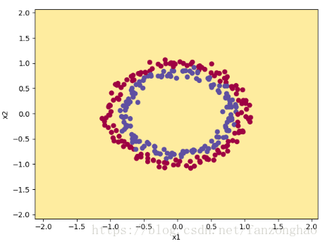
结果2:初始化权重为0~1之间的数的结果


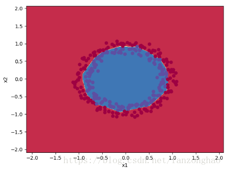
结果3:初始化权重为0~1之间,方差为2/n的结果