版权声明:本文为博主原创文章,未经博主允许不得转载。 https://blog.csdn.net/ocean1171597779/article/details/87971302
# (c) Silvaco Inc., 2013
go atlas
#
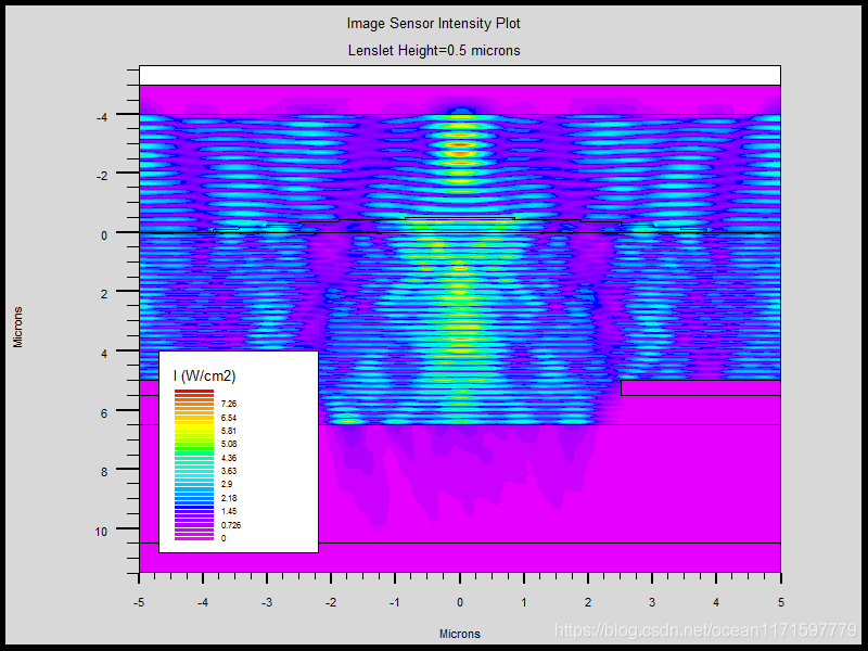
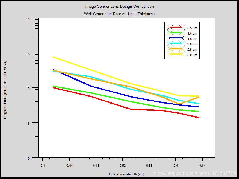
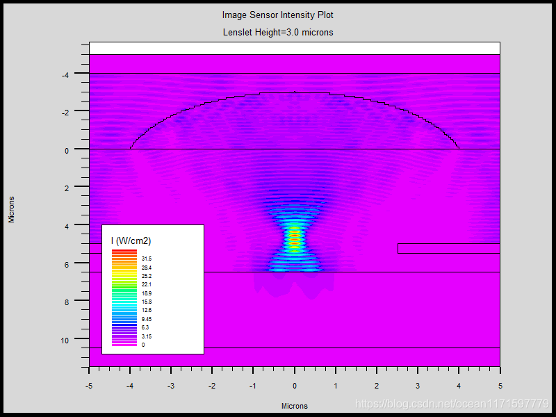
# Lenslet Optimization
# Here we compare several lenslet designs. All lenses for comparison
# are spherical but have different radiuses. The width of the lens
# at the surface is fixed. The lens effectiveness is quantified by the
# integrated photogeneration rate in a box at the detector well.
#
# Case 1:
#
mesh
#
# Structure definition
#
x.m l=-5 s=0.1
x.m l=5 s=0.1
y.m l=0 s=0.25
y.m l=5.0 s=0.05
y.m l=5.5 s=0.05
y.m l=6.5 s=0.05
y.m l=9.5 s=0.1
y.m l=10.5 s=0.1
#
region num=1 silicon y.min=6.5
region num=2 oxide y.max=6.5
region num=3 material=aluminum x.min=-5.0 x.max=-2.5 y.min=5 y.max=5.5
region num=4 material=aluminum x.min=2.5 x.max=5.0 y.min=5 y.max=5.5
#
elec num=1 substrate
elec num=2 material=aluminum x.min=-5.0 x.max=-2.5 y.min=5 y.max=5.5
elec num=3 material=aluminum x.min=2.5 x.max=5.0 y.min=5 y.max=5.5
#
# Background doping
#
doping region=1 unif p.type conc=2e15
#
# Isolation
#
doping region=1 gaus p.type conc=1e18 peak=6.5 char=0.25 x.min=-5.0 x.max=-2.5
doping region=1 gaus p.type conc=1e18 peak=6.5 char=0.25 x.min=2.5 x.max=5.0
#
# Nwell
#
doping region=1 gaus n.type conc=1e16 peak=6.6 char=0.05
#
# Here we set some models. For this analysis these are not too important
# as we are only looking at photogeneration.
#
model srh conmob fldmob print
#
# We choose a high index to reflect light in FDFD.
#
material material=Aluminum real.index=1 imag.index=10
#
# We choose to output optical intensity
#
output opt.int
#
# Here we define the optical source. It is incident normal to the device
# from above. We select spacings
# in time and space. The space step should be a small fraction of the
# wavelength (about 1/20th). We specify to propogate 111 wavelengths.
# At the end of the simulation we output a structure file of the FDTD
# representation.
#
beam num=1 fdtd x.origin=0.0 y.origin=-4.0 angle=90.0 wavelength=0.415 \
td.srate=7 fd.auto prop.leng=10 big.index td.err=0.01 \
td.end td.file="imagesensorex01_1"
#
# Here we specify the spherical lens by index, location and radius.
#
lens plane=0.0 index=1.586 x.loc=0.0 y.loc=15.75 radius=16.25 spheric
#
# We specify perfectly matched layers (PMLs) at the top and the bottom
# to absorb exiting radiation.
#
pml top degree=1 width=1 r90=0.001
pml bottom degree=1 width=1 r90=0.001 material=silicon
#
# We get an initial solution.
#
solve init
#
# Specify 2 carrier solutions
#
method carriers=2
#
# We probe the integrated photogeneration rate in a bounding box around
# the N well.
#
probe name="Gp" photogen fdtd integrate x.min=-2.5 x.max=2.5 y.min=6.5 y.max=7.5
#
# We will capture the output in a log file.
#
log outf=imagesensorex01_1.log
#
# Turn on the light and get a solution
#
# violet
solve b1=0.001 lambda=0.415
# blue
solve b1=0.001 lambda=0.4725
# green
solve b1=0.001 lambda=0.5325
save outf=imagesensorex01_1.str
# yellow
solve b1=0.001 lambda=0.58
# orange
solve b1=0.001 lambda=0.605
# red
solve b1=0.001 lambda=0.635
#
tonyplot imagesensorex01_1.str -set imagesensorex01_1.set
go atlas
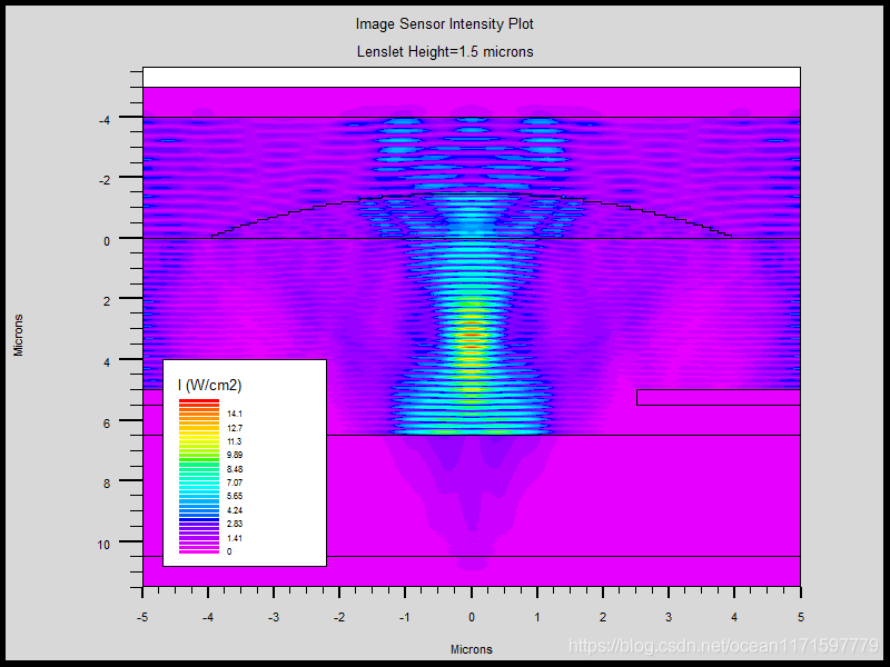
# Case 2:
#
mesh
#
# Structure definition
#
x.m l=-5 s=0.1
x.m l=5 s=0.1
y.m l=0 s=0.25
y.m l=5.0 s=0.05
y.m l=5.5 s=0.05
y.m l=6.5 s=0.05
y.m l=9.5 s=0.1
y.m l=10.5 s=0.1
#
region num=1 silicon y.min=6.5
region num=2 oxide y.max=6.5
region num=3 material=aluminum x.min=-5.0 x.max=-2.5 y.min=5 y.max=5.5
region num=4 material=aluminum x.min=2.5 x.max=5.0 y.min=5 y.max=5.5
#
elec num=1 substrate
elec num=2 material=aluminum x.min=-5.0 x.max=-2.5 y.min=5 y.max=5.5
elec num=3 material=aluminum x.min=2.5 x.max=5.0 y.min=5 y.max=5.5
#
# Background doping
#
doping region=1 unif p.type conc=2e15
#
# Isolation
#
doping region=1 gaus p.type conc=1e18 peak=6.5 char=0.25 x.min=-5.0 x.max=-2.5
doping region=1 gaus p.type conc=1e18 peak=6.5 char=0.25 x.min=2.5 x.max=5.0
#
# Nwell
#
doping region=1 gaus n.type conc=1e16 peak=6.6 char=0.05
#
# Here we set some models. For this analysis these are not too important
# as we are only looking at photogeneration.
#
model srh conmob fldmob print
#
# We choose a high index to reflect light in FDFD.
#
material material=Aluminum real.index=1 imag.index=10
#
# We choose to output optical intensity
#
output opt.int
#
# Here we define the optical source. It is incident normal to the device
# from above. We select spacings
# in time and space. The space step should be a small fraction of the
# wavelength (about 1/20th). We specify to propogate 111 wavelengths.
# At the end of the simulation we output a structure file of the FDTD
# representation.
#
beam num=1 fdtd x.origin=0.0 y.origin=-4.0 angle=90.0 wavelength=0.415 \
td.srate=7 fd.auto prop.leng=10 big.index td.err=0.01 \
td.end td.file="imagesensorex01_2"
#
# Here we specify the spherical lens by index, location and radius.
#
lens plane=0.0 index=1.586 x.loc=0.0 y.loc=7.5 radius=8.5 spheric
#
# We specify perfectly matched layers (PMLs) at the top and the bottom
# to absorb exiting radiation.
#
pml top degree=1 width=1 r90=0.001
pml bottom degree=1 width=1 r90=0.001 material=silicon
#
# We get an initial solution.
#
solve init
#
# Specify 2 carrier solutions
#
method carriers=2
#
# We probe the integrated photogeneration rate in a bounding box around
# the N well.
#
probe name="Gp" photogen fdtd integrate x.min=-2.5 x.max=2.5 y.min=6.5 y.max=7.5
#
# We will capture the output in a log file.
#
log outf=imagesensorex01_2.log
#
# Turn on the light and get a solution
#
# violet
solve b1=0.001 lambda=0.415
# blue
solve b1=0.001 lambda=0.4725
# green
solve b1=0.001 lambda=0.5325
save outf=imagesensorex01_2.str
# yellow
solve b1=0.001 lambda=0.58
# orange
solve b1=0.001 lambda=0.605
# red
solve b1=0.001 lambda=0.635
#
tonyplot imagesensorex01_2.str -set imagesensorex01_2.set
go atlas
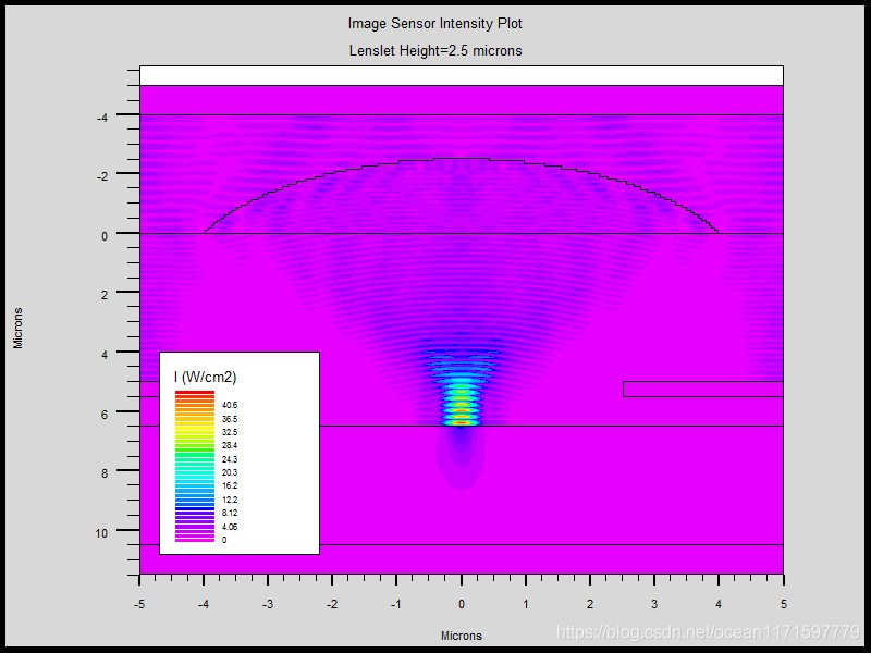
# Case 3:
#
mesh
#
# Structure definition
#
x.m l=-5 s=0.1
x.m l=5 s=0.1
y.m l=0 s=0.25
y.m l=5.0 s=0.05
y.m l=5.5 s=0.05
y.m l=6.5 s=0.05
y.m l=9.5 s=0.1
y.m l=10.5 s=0.1
#
region num=1 silicon y.min=6.5
region num=2 oxide y.max=6.5
region num=3 material=aluminum x.min=-5.0 x.max=-2.5 y.min=5 y.max=5.5
region num=4 material=aluminum x.min=2.5 x.max=5.0 y.min=5 y.max=5.5
#
elec num=1 substrate
elec num=2 material=aluminum x.min=-5.0 x.max=-2.5 y.min=5 y.max=5.5
elec num=3 material=aluminum x.min=2.5 x.max=5.0 y.min=5 y.max=5.5
#
# Background doping
#
doping region=1 unif p.type conc=2e15
#
# Isolation
#
doping region=1 gaus p.type conc=1e18 peak=6.5 char=0.25 x.min=-5.0 x.max=-2.5
doping region=1 gaus p.type conc=1e18 peak=6.5 char=0.25 x.min=2.5 x.max=5.0
#
# Nwell
#
doping region=1 gaus n.type conc=1e16 peak=6.6 char=0.05
#
# Here we set some models. For this analysis these are not too important
# as we are only looking at photogeneration.
#
model srh conmob fldmob print
#
# We choose a high index to reflect light in FDFD.
#
material material=Aluminum real.index=1 imag.index=10
#
# We choose to output optical intensity
#
output opt.int
#
# Here we define the optical source. It is incident normal to the device
# from above. We select spacings
# in time and space. The space step should be a small fraction of the
# wavelength (about 1/20th). We specify to propogate 111 wavelengths.
# At the end of the simulation we output a structure file of the FDTD
# representation.
#
beam num=1 fdtd x.origin=0.0 y.origin=-4.0 angle=90.0 wavelength=0.415 \
td.srate=7 fd.auto prop.leng=10 big.index td.err=0.01 \
td.end td.file="imagesensorex01_3"
#
# Here we specify the spherical lens by index, location and radius.
#
lens plane=0.0 index=1.586 x.loc=0.0 y.loc=4.5833 radius=6.0833 spheric
#
# We specify perfectly matched layers (PMLs) at the top and the bottom
# to absorb exiting radiation.
#
pml top degree=1 width=1 r90=0.001
pml bottom degree=1 width=1 r90=0.001 material=silicon
#
# We get an initial solution.
#
solve init
#
# Specify 2 carrier solutions
#
method carriers=2
#
# We probe the integrated photogeneration rate in a bounding box around
# the N well.
#
probe name="Gp" photogen fdtd integrate x.min=-2.5 x.max=2.5 y.min=6.5 y.max=7.5
#
# We will capture the output in a log file.
#
log outf=imagesensorex01_3.log
#
# Turn on the light and get a solution
#
# violet
solve b1=0.001 lambda=0.415
# blue
solve b1=0.001 lambda=0.4725
# green
solve b1=0.001 lambda=0.5325
save outf=imagesensorex01_3.str
# yellow
solve b1=0.001 lambda=0.58
# orange
solve b1=0.001 lambda=0.605
# red
solve b1=0.001 lambda=0.635
#
tonyplot imagesensorex01_3.str -set imagesensorex01_3.set
go atlas
# Case 4:
#
mesh
#
# Structure definition
#
x.m l=-5 s=0.1
x.m l=5 s=0.1
y.m l=0 s=0.25
y.m l=5.0 s=0.05
y.m l=5.5 s=0.05
y.m l=6.5 s=0.05
y.m l=9.5 s=0.1
y.m l=10.5 s=0.1
#
region num=1 silicon y.min=6.5
region num=2 oxide y.max=6.5
region num=3 material=aluminum x.min=-5.0 x.max=-2.5 y.min=5 y.max=5.5
region num=4 material=aluminum x.min=2.5 x.max=5.0 y.min=5 y.max=5.5
#
elec num=1 substrate
elec num=2 material=aluminum x.min=-5.0 x.max=-2.5 y.min=5 y.max=5.5
elec num=3 material=aluminum x.min=2.5 x.max=5.0 y.min=5 y.max=5.5
#
# Background doping
#
doping region=1 unif p.type conc=2e15
#
# Isolation
#
doping region=1 gaus p.type conc=1e18 peak=6.5 char=0.25 x.min=-5.0 x.max=-2.5
doping region=1 gaus p.type conc=1e18 peak=6.5 char=0.25 x.min=2.5 x.max=5.0
#
# Nwell
#
doping region=1 gaus n.type conc=1e16 peak=6.6 char=0.05
#
# Here we set some models. For this analysis these are not too important
# as we are only looking at photogeneration.
#
model srh conmob fldmob print
#
# We choose a high index to reflect light in FDFD.
#
material material=Aluminum real.index=1 imag.index=10
#
# We choose to output optical intensity
#
output opt.int
#
# Here we define the optical source. It is incident normal to the device
# from above. We select spacings
# in time and space. The space step should be a small fraction of the
# wavelength (about 1/20th). We specify to propogate 111 wavelengths.
# At the end of the simulation we output a structure file of the FDTD
# representation.
#
beam num=1 fdtd x.origin=0.0 y.origin=-4.0 angle=90.0 wavelength=0.415 \
td.srate=7 fd.auto prop.leng=10 big.index td.err=0.01 \
td.end td.file="imagesensorex01_4"
#
# Here we specify the spherical lens by index, location and radius.
#
lens plane=0.0 index=1.586 x.loc=0.0 y.loc=3.0 radius=5.0 spheric
#
# We specify perfectly matched layers (PMLs) at the top and the bottom
# to absorb exiting radiation.
#
pml top degree=1 width=1 r90=0.001
pml bottom degree=1 width=1 r90=0.001 material=silicon
#
# We get an initial solution.
#
solve init
#
# Specify 2 carrier solutions
#
method carriers=2
#
# We probe the integrated photogeneration rate in a bounding box around
# the N well.
#
probe name="Gp" photogen fdtd integrate x.min=-2.5 x.max=2.5 y.min=6.5 y.max=7.5
#
# We will capture the output in a log file.
#
log outf=imagesensorex01_4.log
#
# Turn on the light and get a solution
#
# violet
solve b1=0.001 lambda=0.415
# blue
solve b1=0.001 lambda=0.4725
# green
solve b1=0.001 lambda=0.5325
save outf=imagesensorex01_4.str
# yellow
solve b1=0.001 lambda=0.58
# orange
solve b1=0.001 lambda=0.605
# red
solve b1=0.001 lambda=0.635
#
tonyplot imagesensorex01_4.str -set imagesensorex01_4.set
go atlas
# Case 5:
#
mesh
#
# Structure definition
#
x.m l=-5 s=0.1
x.m l=5 s=0.1
y.m l=0 s=0.25
y.m l=5.0 s=0.05
y.m l=5.5 s=0.05
y.m l=6.5 s=0.05
y.m l=9.5 s=0.1
y.m l=10.5 s=0.1
#
region num=1 silicon y.min=6.5
region num=2 oxide y.max=6.5
region num=3 material=aluminum x.min=-5.0 x.max=-2.5 y.min=5 y.max=5.5
region num=4 material=aluminum x.min=2.5 x.max=5.0 y.min=5 y.max=5.5
#
elec num=1 substrate
elec num=2 material=aluminum x.min=-5.0 x.max=-2.5 y.min=5 y.max=5.5
elec num=3 material=aluminum x.min=2.5 x.max=5.0 y.min=5 y.max=5.5
#
# Background doping
#
doping region=1 unif p.type conc=2e15
#
# Isolation
#
doping region=1 gaus p.type conc=1e18 peak=6.5 char=0.25 x.min=-5.0 x.max=-2.5
doping region=1 gaus p.type conc=1e18 peak=6.5 char=0.25 x.min=2.5 x.max=5.0
#
# Nwell
#
doping region=1 gaus n.type conc=1e16 peak=6.6 char=0.05
#
# Here we set some models. For this analysis these are not too important
# as we are only looking at photogeneration.
#
model srh conmob fldmob print
#
# We choose a high index to reflect light in FDFD.
#
material material=Aluminum real.index=1 imag.index=10
#
# We choose to output optical intensity
#
output opt.int
#
# Here we define the optical source. It is incident normal to the device
# from above. We select spacings
# in time and space. The space step should be a small fraction of the
# wavelength (about 1/20th). We specify to propogate 111 wavelengths.
# At the end of the simulation we output a structure file of the FDTD
# representation.
#
beam num=1 fdtd x.origin=0.0 y.origin=-4.0 angle=90.0 wavelength=0.415 \
td.srate=7 fd.auto prop.leng=10 big.index td.err=0.01 \
td.end td.file="imagesensorex01_5"
#
# Here we specify the spherical lens by index, location and radius.
#
lens plane=0.0 index=1.586 x.loc=0.0 y.loc=1.95 radius=4.45 spheric
#
# We specify perfectly matched layers (PMLs) at the top and the bottom
# to absorb exiting radiation.
#
pml top degree=1 width=1 r90=0.001
pml bottom degree=1 width=1 r90=0.001 material=silicon
#
# We get an initial solution.
#
solve init
#
# Specify 2 carrier solutions
#
method carriers=2
#
# We probe the integrated photogeneration rate in a bounding box around
# the N well.
#
probe name="Gp" photogen fdtd integrate x.min=-2.5 x.max=2.5 y.min=6.5 y.max=7.5
#
# We will capture the output in a log file.
#
log outf=imagesensorex01_5.log
#
# Turn on the light and get a solution
#
# violet
solve b1=0.001 lambda=0.415
# blue
solve b1=0.001 lambda=0.4725
# green
solve b1=0.001 lambda=0.5325
save outf=imagesensorex01_5.str
# yellow
solve b1=0.001 lambda=0.58
# orange
solve b1=0.001 lambda=0.605
# red
solve b1=0.001 lambda=0.635
#
tonyplot imagesensorex01_5.str -set imagesensorex01_5.set
go atlas
# Case 6:
#
mesh
#
# Structure definition
#
x.m l=-5 s=0.1
x.m l=5 s=0.1
y.m l=0 s=0.25
y.m l=5.0 s=0.05
y.m l=5.5 s=0.05
y.m l=6.5 s=0.05
y.m l=9.5 s=0.1
y.m l=10.5 s=0.1
#
region num=1 silicon y.min=6.5
region num=2 oxide y.max=6.5
region num=3 material=aluminum x.min=-5.0 x.max=-2.5 y.min=5 y.max=5.5
region num=4 material=aluminum x.min=2.5 x.max=5.0 y.min=5 y.max=5.5
#
elec num=1 substrate
elec num=2 material=aluminum x.min=-5.0 x.max=-2.5 y.min=5 y.max=5.5
elec num=3 material=aluminum x.min=2.5 x.max=5.0 y.min=5 y.max=5.5
#
# Background doping
#
doping region=1 unif p.type conc=2e15
#
# Isolation
#
doping region=1 gaus p.type conc=1e18 peak=6.5 char=0.25 x.min=-5.0 x.max=-2.5
doping region=1 gaus p.type conc=1e18 peak=6.5 char=0.25 x.min=2.5 x.max=5.0
#
# Nwell
#
doping region=1 gaus n.type conc=1e16 peak=6.6 char=0.05
#
# Here we set some models. For this analysis these are not too important
# as we are only looking at photogeneration.
#
model srh conmob fldmob print
#
# We choose a high index to reflect light in FDFD.
#
material material=Aluminum real.index=1 imag.index=10
#
# We choose to output optical intensity
#
output opt.int
#
# Here we define the optical source. It is incident normal to the device
# from above. We select spacings
# in time and space. The space step should be a small fraction of the
# wavelength (about 1/20th). We specify to propogate 111 wavelengths.
# At the end of the simulation we output a structure file of the FDTD
# representation.
#
beam num=1 fdtd x.origin=0.0 y.origin=-4.0 angle=90.0 wavelength=0.415 \
td.srate=7 fd.auto prop.leng=10 big.index td.err=0.01 \
td.end td.file="imagesensorex01_6"
#
# Here we specify the spherical lens by index, location and radius.
#
lens plane=0.0 index=1.586 x.loc=0.0 y.loc=1.1667 radius=4.1667 spheric
#
# We specify perfectly matched layers (PMLs) at the top and the bottom
# to absorb exiting radiation.
#
pml top degree=1 width=1 r90=0.001
pml bottom degree=1 width=1 r90=0.001 material=silicon
#
# We get an initial solution.
#
solve init
#
# Specify 2 carrier solutions
#
method carriers=2
#
# We probe the integrated photogeneration rate in a bounding box around
# the N well.
#
probe name="Gp" photogen fdtd integrate x.min=-2.5 x.max=2.5 y.min=6.5 y.max=7.5
#
# We will capture the output in a log file.
#
log outf=imagesensorex01_6.log
#
# Turn on the light and get a solution
#
# violet
solve b1=0.001 lambda=0.415
# blue
solve b1=0.001 lambda=0.4725
# green
solve b1=0.001 lambda=0.5325
save outf=imagesensorex01_6.str
# yellow
solve b1=0.001 lambda=0.58
# orange
solve b1=0.001 lambda=0.605
# red
solve b1=0.001 lambda=0.635
#
tonyplot imagesensorex01_6.str -set imagesensorex01_6.set
tonyplot -overlay imagesensorex01_1.log imagesensorex01_2.log imagesensorex01_3.log imagesensorex01_4.log imagesensorex01_5.log imagesensorex01_6.log -set imagesensorex01_7.set
quit