文章目录
2 K-近邻算法 & 3 决策树
4 基于概率论的分类方法:朴素贝叶斯
4.5 使用Python进行文本分类
4.5.1 准备数据:从文本中构建词向量
我们把文本看成单词向量或者词条向量,也就是说将句子转换为向量。创建新文件bayesCopy.py
# 创建一个实验样本
def loadDataSet():
    postingList=[['my', 'dog', 'has', 'flea', 'problems', 'help', 'please'],
                 ['maybe', 'not', 'take', 'him', 'to', 'dog', 'park', 'stupid'],
                 ['my', 'dalmation', 'is', 'so', 'cute', 'I', 'love', 'him'],
                 ['stop', 'posting', 'stupid', 'worthless', 'garbage'],
                 ['mr', 'licks', 'ate', 'my', 'steak', 'how', 'to', 'stop', 'him'],
                 ['quit', 'buying', 'worthless', 'dog', 'food', 'stupid']]
    classVec = [0,1,0,1,0,1]    #1 is abusive, 0 not
    return postingList,classVec
# 创建一个包含在所有文档中出现的不重复词的列表
def createVocabList(dataSet):
    vocabSet = set([])
    for document in dataSet:
        vocabSet = vocabSet | set(document)
    return list(vocabSet)
# 检测输入的词是否在词汇表中,输出文档向量
def setOfWords2Vec(vocabList, inputSet):
    returnVec = [0]*len(vocabList)
    # print(returnVec)
    # print(inputSet)
    for word in inputSet:
        if word in vocabList:
            returnVec[vocabList.index(word)] = 1
        else:   print("the word: %s is not in my Vocabulary!"%word)
    return returnVec
测试结果:
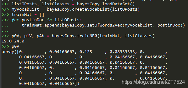
from mechineLearning.Ch04 import bayesCopy
listOPosts, listClasses = bayesCopy.loadDataSet()
myVocabList = bayesCopy.createVocabList(listOPosts)
myVocabList
['quit', 'flea', 'my', 'him', 'worthless', 'ate', 'garbage', 'buying', 'dog', 'licks', 'has', 'please', 'steak', 'cute', 'not', 'mr', 'maybe', 'stop', 'dalmation', 'is', 'food', 'park', 'so', 'posting', 'how', 'take', 'problems', 'to', 'stupid', 'love', 'help', 'I']
bayesCopy.setOfWords2Vec(myVocabList, listOPosts[0])
[0, 1, 1, 0, 0, 0, 0, 0, 1, 0, 1, 1, 0, 0, 0, 0, 0, 0, 0, 0, 0, 0, 0, 0, 0, 0, 1, 0, 0, 0, 1, 0]
bayesCopy.setOfWords2Vec(myVocabList, listOPosts[3])
[0, 0, 0, 0, 1, 0, 1, 0, 0, 0, 0, 0, 0, 0, 0, 0, 0, 1, 0, 0, 0, 0, 0, 1, 0, 0, 0, 0, 1, 0, 0, 0]
4.5.2 训练算法:从词向量计算频率
朴素贝叶斯分类器训练函数
# 朴素贝叶斯分类器训练函数
def trainNB0(trainMatrix, trainCategory):
    numTrainDocs = len(trainMatrix)
    numWords = len(trainMatrix[0])
    pAbusive = sum(trainCategory)/float(numTrainDocs)
    p0Num = np.zeros(numWords); p1Num = np.zeros(numWords)
    p0Denom = 0.0; p1Denom = 0.0
    for i in range(numTrainDocs):
        if trainCategory[i] == 1:
            p1Num += trainMatrix[i]
            p1Denom += sum(trainMatrix[i])
        else:
            # print(trainMatrix[i])
            p0Num += trainMatrix[i]
            p0Denom += sum(trainMatrix[i])
            # print()
    print(p1Denom, p0Denom)
    p1Vect = p1Num/p1Denom
    p0Vect = p0Num/p0Denom
    return p0Vect, p1Vect, pAbusive
计算p(w|c),上述函数是在确定类别的情况下,直接计算出现频次。
测试结果:
4.5.3 测试算法: 根据现实情况修改分类器
避免分母或者其中某一分子为零而导致整个概率为零;为解决下溢出问题;
在trainNB0(),函数中修改相应代码。
# 避免分母或者其中某一分子为零而导致整个概率为零
    p0Num = np.ones(numWords);    p1Num = np.ones(numWords)
    p0Denom = 1.0;    p1Denom = 2.0

    p1Vect = np.log(p1Num/p1Denom)
    p0Vect = np.log(p0Num/p0Denom)
朴素贝叶斯分类函数:
# 朴素贝叶斯分类函数
def classifyNB(vec2Classify, p0Vec, p1Vec, pClass1):
    p1 = sum(vec2Classify * p1Vec) + np.log(pClass1)
    p0 = sum(vec2Classify * p0Vec) + np.log(pClass1)
    if p1 > p0:
        return 1
    else:
        return 0

def testingNB():
    listOPosts, listClasses = loadDataSet()
    myVocabList = createVocabList(listOPosts)
    trainMat = []
    for postinDoc in listOPosts:
        trainMat.append(setOfWords2Vec(myVocabList, postinDoc))
    p0V, p1V, pAb = trainNB0(np.array(trainMat), np.array(listClasses))
    testEntry = ['love', 'my', 'dalmation']
    thisDoc = np.array(setOfWords2Vec(myVocabList, testEntry))
    print(testEntry, 'classified as: ', classifyNB(thisDoc, p0V, p1V, pAb))
    testEntry = ['stupid', 'garbage']
    thisDoc = np.array(setOfWords2Vec(myVocabList, testEntry))
    print(testEntry, 'classified as: ', classifyNB(thisDoc, p0V, p1V, pAb))
    testEntry = ['my', 'stop']
    thisDoc = np.array(setOfWords2Vec(myVocabList, testEntry))
    print(testEntry, 'classified as: ', classifyNB(thisDoc, p0V, p1V, pAb))
测试结果:
bayesCopy.testingNB()
21.0 25.0
['love', 'my', 'dalmation'] classified as:  0
['stupid', 'garbage'] classified as:  1
['my', 'stop'] classified as:  0
4.5.4 准备数据:文档词袋模型
我们将每个词的出现是否作为一个特征,这可以被描述为词集模型;
如果一个词在文档中不止出现一次,这可能意味着包含该词是否出现在文档中所不能表达的某种信息这种方法被称为词袋模型。
因此,我们需要之前的函数setOfWords2Vec(),进行修改。
# 词袋模型
def bigOfWords2Vec(vocabList, inputSet):
    returnVec = [0]*len(vocabList)
    for word in inputSet:
        if word in vocabList:
            returnVec[vocabList.index(word)] += 1
    return returnVec
4.6 示例:使用朴素贝叶斯过滤垃圾邮件
4.6.1 准备数据:切分文本
# 文件解析
def textParse(bigString):
    import re
    listOfTokens = re.split(r'\W*', bigString)
    return [tok.lower() for tok in listOfTokens if len(tok) > 2]
4.6.2 测试算法:使用朴素贝叶斯进行交叉验证
注意:
- 源文件给的
Ch04/email/ham/24.txt中有系统默认的编码方式所不能识别的字符,运行程序会报如下错误:UnicodeDecodeError: 'gbk' codec can't decode byte 0xbd in position 198: illegal multibyte sequence。此时,我们只需打开文本编译器(如:pycharm)删除不能识别的字符即可。 - 处理错误
TypeError: 'range' object doesn't support item deletion。
原因分析:python3.x range返回的是range对象,不返回数组对象;
因此我们只需修改trainingSet = list(range(50))就可以了。
# 完整的垃圾邮件测试函数
def spamTest():
    docList = []; classList = []; fullTest = []
    for i in range(1, 26):
        wordList = textParse(open(r'mechineLearning/Ch04/email/ham/%d.txt'% i,).read())

        docList.append(wordList)
        fullTest.extend(wordList)
        classList.append(1)
        wordList = textParse(open(r'mechineLearning/Ch04/email/spam/%d.txt'% i).read())
        docList.append(wordList)
        fullTest.extend(wordList)
        classList.append(0)
    vocabList = createVocabList(docList)
    trainingSet = list(range(50)); testSet = []
    for i in range(10):
        randIndex = int(np.random.uniform(0, len(trainingSet)))
        testSet.append(trainingSet[randIndex])
        del[trainingSet[randIndex]]
    trainMat = []; trainClasses = []
    # print(list(trainingSet))
    for docIndex in trainingSet:
        trainMat.append(setOfWords2Vec(vocabList, docList[docIndex]))
        trainClasses.append(classList[docIndex])
    p0V,p1V,pSpam = trainNB0(np.array(trainMat), np.array(trainClasses))
    errorCount = 0
    for docIndex in testSet:
        wordVector = setOfWords2Vec(vocabList, docList[docIndex])
        if classifyNB(wordVector, p0V,p1V,pSpam) != classList[docIndex]:
            errorCount += 1
        print ("classification error",docList[docIndex])
    print('the error rate is: ', float(errorCount)/len(testSet))
测试结果:
由于是随机选取的十封邮件,所有测试结果会有所不同。
bayesCopy.spamTest()
classification error ['benoit', 'mandelbrot', '1924', '2010', 'benoit', 'mandelbrot', '1924', '2010', 'wilmott', 'team', 'benoit', 'mandelbrot', 'the', 'mathematician', 'the', 'father', 'fractal', 'mathematics', 'and', 'advocate', 'more', 'sophisticated', 'modelling', 'quantitative', 'finance', 'died', '14th', 'october', '2010', 'aged', 'wilmott', 'magazine', 'has', 'often', 'featured', 'mandelbrot', 'his', 'ideas', 'and', 'the', 'work', 'others', 'inspired', 'his', 'fundamental', 'insights', 'you', 'must', 'logged', 'view', 'these', 'articles', 'from', 'past', 'issues', 'wilmott', 'magazine']
the error rate is:  0.1
bayesCopy.spamTest()
the error rate is:  0.0
4.7 使用朴素贝叶斯分类器从广告中获取区域倾向
5 Logistic回归
5.2 基于最优化方法的最佳回归系数确定
5.2.1 梯度上升法
梯度上升法主要思想:要找到函数的最大值,最好的方法是沿着该函数的梯度方向探寻。
5.2.2 训练算法:使用梯度上升找到最佳参数
Logistic回归梯度上升优化算法。
import numpy as np
# 读取文本中的数据
def loadDataSet():
    dataMat = []; labelMat = []
    fr = open('mechineLearning/Ch05/testSet.txt')
    for line in fr.readlines():
        lineArr = line.strip().split()
        dataMat.append([1.0,float(lineArr[0]),float(lineArr[1])])
        labelMat.append(int(lineArr[2]))
    return dataMat, labelMat

def sigmoid(inX):
    return 1.0/(1+np.exp(-inX))
# 确定最佳参数
def gradAscent(dataMatIn, classLabels):
    dataMatrix = np.mat(dataMatIn)
    labelsMat = np.mat(classLabels).transpose()
    m, n = np.shape(dataMatrix)
    # 我们将这里的移动量成为步长,记为 alpha
    alpha = 0.001
    maxCycles = 500
    # 参数变量
    weights = np.ones((n,1))
    for k in range(maxCycles):
        h = sigmoid(dataMatrix*weights)
        error = (labelsMat -h)
        # 这里是通过一个人为确定的一个函数(平方损失函数),来确定参数
        weights = weights + alpha * dataMatrix.transpose() * error
    return weights
weights = weights + alpha * dataMatrix.transpose() * error推导过程:
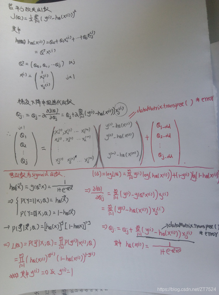
图片来源
在最优化方法中,这些梯度下降(上升)函数往往可以有我们自己来指定。只要是最优就可以。
测试结果,这里是在pycharm交互式命令行测试。
from mechineLearning.Ch05 import logResgresCopy
dataArr, labelMat = logResgresCopy.loadDataSet()
logResgresCopy.gradAscent(dataArr, labelMat)
matrix([[ 4.12414349],
        [ 0.48007329],
        [-0.6168482 ]])
5.2.3 分析数据: 画出决策边界
画出数据集和Logistic回归最佳拟合直线的函数
# 画出决策分界线
def plotBestFit(weights):
    import matplotlib.pyplot as plt
    dataMat,labelMat = loadDataSet()
    dataArr = np.array(dataMat)
    n = np.shape(dataArr)[0]
    xcord1 = []; ycord1 = []
    xcord2 = []; ycord2 = []
    for i in range(n):
        if int(labelMat[i]) == 1:
            xcord1.append(dataArr[i,1])
            ycord1.append(dataArr[i,2])
        else:
            xcord2.append(dataArr[i,1])
            ycord2.append(dataArr[i,2])
    fig = plt.figure(num=1)
    ax = fig.add_subplot(111)
    # ax.scatter(xcord1,ycord1,s=30,c='red',marker='s')
    # ax.scatter(xcord2,ycord2,s=30,c='green')
    plt.scatter(xcord1, ycord1, s=30, c='red', marker='s')
    plt.scatter(xcord2, ycord2, s=30, c='green')
    x = np.arange(-3.0, 3.0, 0.1)
    weights = np.array(weights)
    y = (-weights[0]-weights[1]*x)/weights[2]
    ax.plot(x,y)
    plt.xlabel('X1'); plt.ylabel('X2')
    plt.show()
测试结果:
weights = logResgresCopy.gradAscent(dataArr, labelMat)
logResgresCopy.plotBestFit(weights.getA())
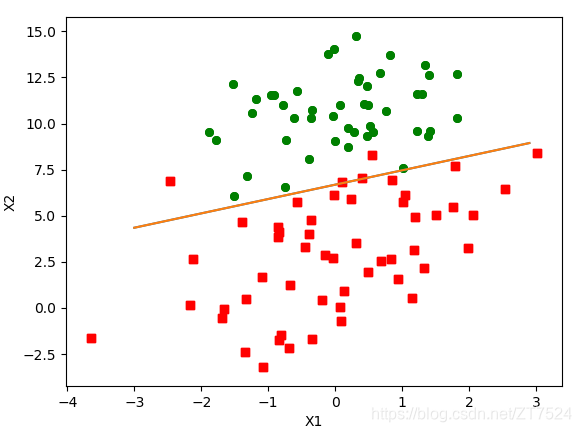
**注意:**这里使用getA()函数将矩阵转为数组,否则会出现x,y维数不同,无法绘制图像
5.2.4 训练算法:随机梯度上升
梯度上升算法在每次更新回归系数时都需要遍历整个数据集,该方法如果处理的样本和特征太多,那么该方法的计算复杂度就太高了。
为此,可以将该方法进行改进,改进方法是每次仅使用一个样本点来更新回归函数,该方法称为随机梯度上升算法。
# 随机梯度上升
def stocGradAscent0(dataMatrix, classLabels):
    m, n = np.shape(dataMatrix)
    alpha = 0.01
    weights = np.ones(n)
    for i in range(m):
        h = sigmoid(sum(dataMatrix[i]*weights))
        error = classLabels[i] - h
        weights = weights + alpha*error*dataMatrix[i]
    return weights
改进的随机梯度上升算法。
# 改进的随机梯度上升算法
def stocGradAscent1(dataMatrix, classLabels, numIter=150):
    m,n = np.shape(dataMatrix)
    weights = np.ones(n)   #initialize to all ones
    for j in range(numIter):
        dataIndex = list(range(m))
        for i in range(m):
            alpha = 4/(1.0+j+i)+0.0001    #apha decreases with iteration, does not
            randIndex = int(np.random.uniform(0,len(dataIndex)))#go to 0 because of the constant
            h = sigmoid(sum(dataMatrix[randIndex]*weights))
            error = classLabels[randIndex] - h
            weights = weights + alpha * error * dataMatrix[randIndex]
            del(dataIndex[randIndex])
    return weights
5.3 示例:从疝气病症预测病马的死亡率
5.3.2 测试算法:用Logistic回归进行分类
Logistic回归分类函数
# 用Logistic回归进行分类
def classifyVector(inX, weights):
    prob = sigmoid(sum(inX * weights))
    if prob > 0.5:
        return 1.0
    else:
        return 0.0


def colicTest():
    frTrain = open('mechineLearning/Ch05/horseColicTraining.txt')
    frTest = open('mechineLearning/Ch05/horseColicTest.txt')
    trainingSet = []
    trainingLabels = []
    for line in frTrain.readlines():
        currLine = line.strip().split('\t')
        lineArr = []
        for i in range(21):
            lineArr.append(float(currLine[i]))
        trainingSet.append(lineArr)
        trainingLabels.append(float(currLine[21]))
    trainWeights = stocGradAscent1(np.array(trainingSet), trainingLabels, 1000)
    errorCount = 0;
    numTestVec = 0.0
    for line in frTest.readlines():
        numTestVec += 1.0
        currLine = line.strip().split('\t')
        lineArr = []
        for i in range(21):
            lineArr.append(float(currLine[i]))
        if int(classifyVector(np.array(lineArr), trainWeights)) != int(currLine[21]):
            errorCount += 1
    errorRate = (float(errorCount) / numTestVec)
    print("the error rate of this test is: %f" % errorRate)
    return errorRate
def multiTest():
    numTests = 10
    errorSum = 0.0
    for k in range(numTests):
        errorSum += colicTest()
    print("after %d iterations the average error rate is: %f"
          % (numTests, errorSum / float(numTests)))
测试结果:
logResgresCopy.multiTest()
E:\Users\Administrator\PycharmProjects\TestCases\mechineLearning\Ch05\logResgresCopy.py:17: RuntimeWarning: overflow encountered in exp
  return 1.0/(1+np.exp(-inX))
the error rate of this test is: 0.328358
the error rate of this test is: 0.373134
the error rate of this test is: 0.328358
the error rate of this test is: 0.432836
the error rate of this test is: 0.298507
the error rate of this test is: 0.283582
the error rate of this test is: 0.328358
the error rate of this test is: 0.373134
the error rate of this test is: 0.402985
the error rate of this test is: 0.283582
after 10 iterations the average error rate is: 0.343284