引言
本篇笔记紧接上文,主要是上一篇看写了快2w字,再去接入代码感觉有点不太妙,后台都崩了好几次,因为内存不足,那就正好将内容分开来,可以水两篇,另外也给脑子放个假,最近事情有点多,思绪都有些乱,跳出原来框架束缚,刚好这篇自由发挥。那么话不多说,上节博文为:
GNN(图神经网络)
该节对应上篇开头介绍GNN的标题,是使用MLP作为分类器来实现图的分类,但我在找资料的时候发现一个很有趣的东西,是2021年发表的一篇为《Graph-MLP: Node Classification without Message Passing in Graph》的论文,按理来说,这东西不应该是很早之前就有尝试嘛?但github上star量最高的也是这篇,我看了下感觉还不错,于是就复现这个了。
论文里的设计框架如下图所示:
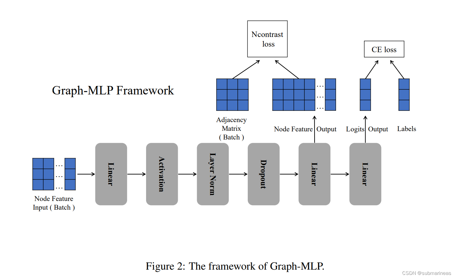
它的整个算法过程为:
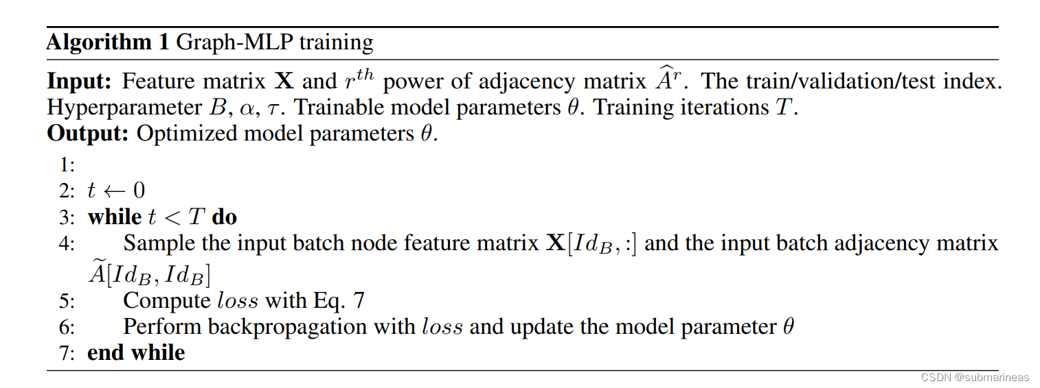
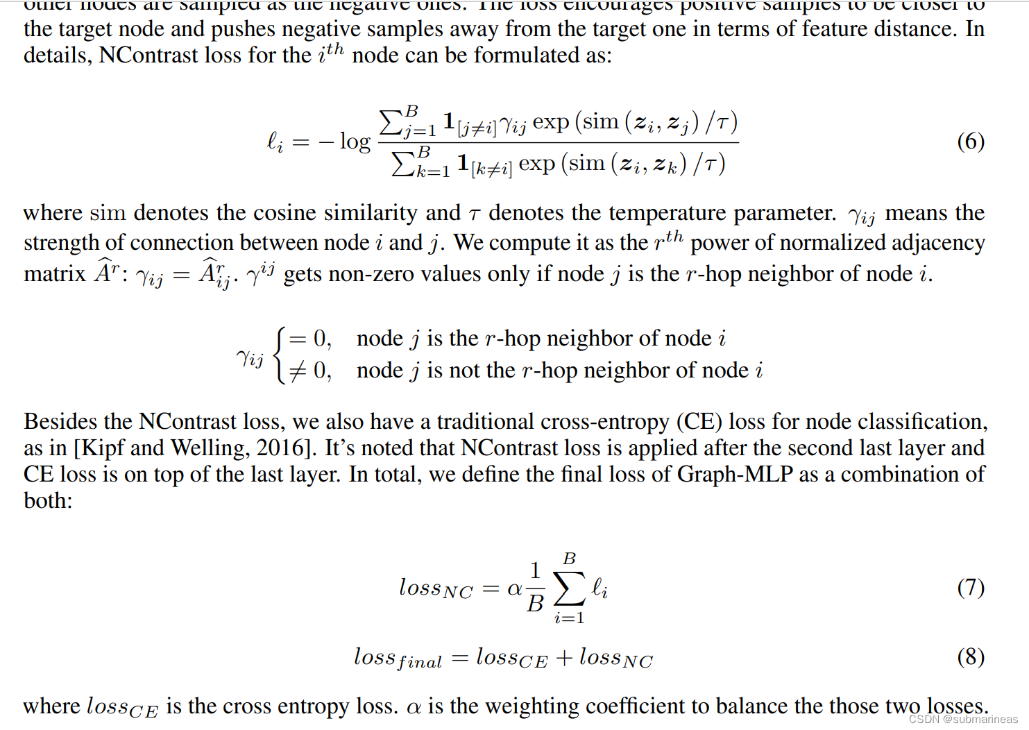
它整个框架加算法给我的感觉非常简单,甚至有点出乎意料,大道至简。我感觉比较创新的地方在Ncontrast loss,即:
不太清楚为啥最终分数会比GCN高,可能这就是神来之笔吧,另外我GCN也还没跑几次,主要是这几天写推导的时候才有的想法,不好做评价。于是我就去看了代码,结果真如论文里写得那样,挺简单的,模型为:
class Mlp(nn.Module):
    def __init__(self, input_dim, hid_dim, dropout):
        super(Mlp, self).__init__()
        self.fc1 = Linear(input_dim, hid_dim)
        self.fc2 = Linear(hid_dim, hid_dim)
        self.act_fn = torch.nn.functional.gelu
        self._init_weights()

        self.dropout = Dropout(dropout)
        self.layernorm = LayerNorm(hid_dim, eps=1e-6)

    def _init_weights(self):
        nn.init.xavier_uniform_(self.fc1.weight)
        nn.init.xavier_uniform_(self.fc2.weight)
        nn.init.normal_(self.fc1.bias, std=1e-6)
        nn.init.normal_(self.fc2.bias, std=1e-6)

    def forward(self, x):
        x = self.fc1(x)
        x = self.act_fn(x)
        x = self.layernorm(x)
        x = self.dropout(x)
        x = self.fc2(x)
        return x
主要的训练代码为:
def train():
    features_batch, adj_label_batch = get_batch(batch_size=args.batch_size)
    model.train()
    optimizer.zero_grad()
    output, x_dis = model(features_batch)
    loss_train_class = F.nll_loss(output[idx_train], labels[idx_train])
    loss_Ncontrast = Ncontrast(x_dis, adj_label_batch, tau = args.tau)
    loss_train = loss_train_class + loss_Ncontrast * args.alpha
    acc_train = accuracy(output[idx_train], labels[idx_train])
    loss_train.backward()
    optimizer.step()
    return
然后我啥环境都没装,直接开跑,启动run.sh,该sh脚本为:
## cora
python3 train.py --lr=0.001 --weight_decay=5e-3 --data=cora --alpha=10.0 --hidden=256 --batch_size=2000 --order=2 --tau=2

## citeseer
python3 train.py --lr=0.001 --weight_decay=5e-3 --data=citeseer --alpha=1.0 --hidden=256 --batch_size=2000 --order=2 --tau=0.5

## pubmed
python3 train.py --lr=0.1 --weight_decay=5e-3 --data=pubmed --alpha=100 --hidden=256 --batch_size=2000 --order=2 --tau=1
然后训练代码没加保存模型,我因为这仨数据集长啥样都不太清楚,也就看看模型结构和最终的复现结果了,作者写在了log.txt中,对比基本一致:
# 作者的测试结果
tau,order,batch_size,hidden,alpha,lr,weight_decay,data,test_acc
2.0,2,2000,256,10.0,0.001,0.005,cora,0.801
tau,order,batch_size,hidden,alpha,lr,weight_decay,data,test_acc
0.5,2,2000,256,1.0,0.001,0.005,citeseer,0.724
tau,order,batch_size,hidden,alpha,lr,weight_decay,data,test_acc
1.0,2,2000,256,100.0,0.1,0.005,pubmed,0.796

# 我的测试结果
tau,order,batch_size,hidden,alpha,lr,weight_decay,data,test_acc
2.0,2,2000,256,10.0,0.001,0.005,cora,0.804
tau,order,batch_size,hidden,alpha,lr,weight_decay,data,test_acc
0.5,2,2000,256,1.0,0.001,0.005,citeseer,0.73
tau,order,batch_size,hidden,alpha,lr,weight_decay,data,test_acc
1.0,2,2000,256,100.0,0.1,0.005,pubmed,0.8
上面为作者预留的数据,下面为我的测试结果,整个过程我都感觉比较神奇,另外就是也有所怀疑,因为我之前文章就有被坑过,在图嵌入里我去复现graphGAN,发现根本跑不出来哪怕一次比较接近的结果,跑知乎逛了一圈,结果看到已经有人把graphGAN作者挂出来吊了,该作者好像依然我行我素,我表示心里有数。
同样,这里我也去查了一下,发现好像原作者有在知乎开贴去回复出现的一些问题,原帖为:

评论区我大概看了一下,有很多提出质疑的,但都一一进行了回复,另外,就现在2023年,有人针对论文的一些不足进行了修复重新复现,得出的结果有所降低,但不算太大,那该种算法我感觉确实有一定可信度,论文与代码都在上述知乎链接中。
GCN:Spectral CNN
上一篇中第二节用频域和空域去将CNN进一步转化成GCN,讲到最开始的GCN其实还是叫spectral CNN,即利用谱域(频域)去实现CNN,底层原理其实就是拉普拉斯的谱分解,这里参考https://github.com/Ivan0131/gcn_demo的代码。
首先,空域卷积的代码为:
class SpatialConvolution(layers.Layer):
    def __init__(self, graph, fin, fout, w_init):
        super(SpatialConvolution, self).__init__()
        # 初始化卷积层参数
        self.fin = fin
        self.fout = fout
        self.num_node = graph.shape[0]
        # 初始化权重
        w_init = w_init(stddev=np.sqrt(2.0/self.fin))
        # 获取非零元素的坐标
        nonzero_inds = np.stack(np.nonzero(graph), axis=1)
        # 初始化权重参数
        weights = tf.Variable(initial_value=w_init(shape=(fin*fout*len(nonzero_inds), ),
                                                  dtype='float32'),
                             trainable=True)
        # 构建权重的非零坐标
        indices = []
        for i in range(fin):
            for j in range(fout):
                fin_ind = np.repeat([[i]], repeats=len(nonzero_inds), axis=0)
                fout_ind = np.repeat([[j]], repeats=len(nonzero_inds), axis=0)
                new_nonzero_inds = np.concatenate([fout_ind, nonzero_inds, fin_ind], axis=1)
                indices.append(new_nonzero_inds)
        indices = np.concatenate(indices, axis=0)

        # 构建稀疏矩阵
        F = tf.sparse.SparseTensor(indices, tf.identity(weights), (fout, self.num_node, self.num_node, fin))

        # 将稀疏矩阵转置并重塑形状
        self.F_tran_reshape = tf.sparse.reorder(tf.sparse.reshape(F, shape=(fout*self.num_node, self.num_node*fin)))

    def call(self, inputs):
        # 调整输入的形状
        inputs_reshape = tf.transpose(tf.reshape(inputs, shape=(-1, self.fin*self.num_node)))

        # 进行卷积计算并使用ReLU激活函数
        c1 = tf.sparse.sparse_dense_matmul(self.F_tran_reshape, inputs_reshape)
        output = tf.nn.relu(c1)
        # 调整输出的形状
        output = tf.reshape(tf.transpose(output), (-1, self.num_node, self.fout))
        return output
频域卷积的代码为:
class SpectralConvolution(layers.Layer):
    def __init__(self, graph, fin, fout, n_component, w_init):
        super(SpectralConvolution, self).__init__()
        """
        # graph: 邻接矩阵
        # fin: 输入特征的维度
        # fout: 输出特征的维度
        # n_component: 保留的特征向量个数
        # w_init: 权重初始化方式
        """
        self.num_node = graph.shape[0]
        self.fin = fin
        self.fout = fout
        self.n_component = n_component
        w_init = w_init(stddev=np.sqrt(2.0/self.fin)) # 使用高斯分布

        # 计算拉普拉斯矩阵,并计算其特征值和特征向量
        laplacian_graph = csgraph.laplacian(graph, normed=False)
        eigen_value, eigen_vector = np.linalg.eig(laplacian_graph.todense())

        # 将特征值和特征向量按特征值从大到小排序,取前n_component个
        idx = eigen_value.argsort()[::-1]
        eigen_value = eigen_value[idx][-self.n_component:]
        eigen_vector = eigen_vector[:,idx][:, -self.n_component:]

        # 转置后得到特征向量矩阵
        self.u = eigen_vector.T

        weights = tf.Variable(initial_value=w_init(shape=(fin*fout*self.n_component, ),
                                                  dtype='float32'),
                             trainable=True)
        indices = []

        # 构建权重的非零坐标
        for i in range(fin):
            for j in range(fout):
                fin_ind = np.repeat([[i]], repeats=self.n_component, axis=0)
                fout_ind = np.repeat([[i]], repeats=self.n_component, axis=0)
                nonzero_inds = np.array([[k, k] for k in range(self.n_component)], dtype=np.int32)
                new_nonzero_inds = np.concatenate([fout_ind, nonzero_inds, fin_ind], axis=1)
                indices.append(new_nonzero_inds)
        indices = np.concatenate(indices, axis=0)

        # 定义稀疏张量,使用之前构建好的非零位置坐标和权重
        F = tf.sparse.SparseTensor(indices, tf.identity(weights), (fout, self.n_component, self.n_component, fin))

        # 将稀疏张量转置并拉成二维张量
        self.F_tran_reshape = tf.sparse.reorder(tf.sparse.reshape(F, shape=(fout*self.n_component, self.n_component*fin)))

    def call(self, inputs):
        # 对输入特征进行傅里叶变换
        inputs_spectral = tf.tensordot(inputs, self.u, axes=[[1], [1]])
        inputs_spectral_reshape = tf.transpose(tf.reshape(inputs_spectral, shape=(-1, self.fin*self.n_component)))

        # 将输入特征和权重矩阵 F 相乘
        F_output = tf.transpose(tf.sparse.sparse_dense_matmul(self.F_tran_reshape, inputs_spectral_reshape))
        F_output = tf.reshape(F_output, (-1, self.fout, self.n_component))

        # 对输出进行傅里叶逆变换
        c1 = tf.transpose(tf.tensordot(F_output, self.u, axes=[[2], [0]]), perm=[0, 2, 1])
        output = tf.nn.relu(c1)
        return output
然后其它的就是建立模型加入优化器等参数进行训练,就不再引述了,都在该GitHub项目中,这里以频域为例:
model = SpectralGCN(W_sample)
model.compile(optimizer, loss=loss_fn, metrics=metrics)
model.fit(x_train_sample, y_train, epochs=20, batch_size=128, validation_data=(x_test_sample, y_test))
"""
Epoch 1/20
469/469 [==============================] - 4s 8ms/step - loss: 0.9142 - sparse_categorical_accuracy: 0.7862 - val_loss: 0.5303 - val_sparse_categorical_accuracy: 0.8670
Epoch 2/20
469/469 [==============================] - 4s 8ms/step - loss: 0.4821 - sparse_categorical_accuracy: 0.8703 - val_loss: 0.4169 - val_sparse_categorical_accuracy: 0.8862
......
Epoch 19/20
469/469 [==============================] - 4s 8ms/step - loss: 0.2545 - sparse_categorical_accuracy: 0.9226 - val_loss: 0.2674 - val_sparse_categorical_accuracy: 0.9209
Epoch 20/20
469/469 [==============================] - 4s 8ms/step - loss: 0.2523 - sparse_categorical_accuracy: 0.9237 - val_loss: 0.2664 - val_sparse_categorical_accuracy: 0.9201
<keras.callbacks.History at 0x7f29ac03a130>
"""
空域也是基本一致的代码,不过作者加了自造的avg pooling,看起来感觉还行,也能更好的在二维上可视化,如下图所示:
从图来讲,我觉得还行,没啥问题,但从迭代的epochs数据,因为时间关系,我把50改成了20,看作者跑的原数据来讲,确实跟论文中的有差距,这里也可以去作者的知乎看他的评价。
GCN:ChebNet
此节使用的切比雪夫优化GCN,论文作者有将代码开源在github,链接为:
https://github.com/mdeff/cnn_graph
该项目中,作者除了对 MNIST 数据集做了试验外,还对 20NEWS做了类似的操作,但比较坑的是,因为项目是2017年的,按照GitHub中源文档写得那样,根本跑不起来了,我也是搞了半天发现不对, MNIST 还能调试下,另一个除非重构,或者完全将全部包退回2017年,不然积重难返,后面会大概提一下具体思路吧。
不得不说,6、7年前的代码,作者看起来在notebook上花了大量功夫,每一段都做了详细说明,我也就不做补充说明了,这里的模型在lib/model下面的cgcnn,整个模型架构为:
class cgcnn(base_model):
    """
    Graph CNN which uses the Chebyshev approximation.
    The following are hyper-parameters of graph convolutional layers.
    They are lists, which length is equal to the number of gconv layers.
        F: Number of features.
        K: List of polynomial orders, i.e. filter sizes or number of hopes.
        p: Pooling size.
           Should be 1 (no pooling) or a power of 2 (reduction by 2 at each coarser level).
           Beware to have coarsened enough.
    L: List of Graph Laplacians. Size M x M. One per coarsening level.
    The following are hyper-parameters of fully connected layers.
    They are lists, which length is equal to the number of fc layers.
        M: Number of features per sample, i.e. number of hidden neurons.
           The last layer is the softmax, i.e. M[-1] is the number of classes.

    The following are choices of implementation for various blocks.
        filter: filtering operation, e.g. chebyshev5, lanczos2 etc.
        brelu: bias and relu, e.g. b1relu or b2relu.
        pool: pooling, e.g. mpool1.

    Training parameters:
        num_epochs:    Number of training epochs.
        learning_rate: Initial learning rate.
        decay_rate:    Base of exponential decay. No decay with 1.
        decay_steps:   Number of steps after which the learning rate decays.
        momentum:      Momentum. 0 indicates no momentum.
    Regularization parameters:
        regularization: L2 regularizations of weights and biases.
        dropout:        Dropout (fc layers): probability to keep hidden neurons. No dropout with 1.
        batch_size:     Batch size. Must divide evenly into the dataset sizes.
        eval_frequency: Number of steps between evaluations.
    Directories:
        dir_name: Name for directories (summaries and model parameters).
    """
实现 Chebyshev 谱图卷积层的代码为:
    def chebyshev5(self, x, L, Fout, K):
        N, M, Fin = x.get_shape()
        N, M, Fin = int(N), int(M), int(Fin)
        # Rescale Laplacian and store as a TF sparse tensor. Copy to not modify the shared L.
        L = scipy.sparse.csr_matrix(L)
        L = graph.rescale_L(L, lmax=2)
        L = L.tocoo()
        indices = np.column_stack((L.row, L.col))
        L = tf.SparseTensor(indices, L.data, L.shape)
        L = tf.sparse_reorder(L)
        # Transform to Chebyshev basis
        x0 = tf.transpose(x, perm=[1, 2, 0])  # M x Fin x N
        x0 = tf.reshape(x0, [M, Fin*N])  # M x Fin*N
        x = tf.expand_dims(x0, 0)  # 1 x M x Fin*N
        def concat(x, x_):
            x_ = tf.expand_dims(x_, 0)  # 1 x M x Fin*N
            return tf.concat([x, x_], axis=0)  # K x M x Fin*N
        if K > 1:
            x1 = tf.sparse_tensor_dense_matmul(L, x0)
            x = concat(x, x1)
        for k in range(2, K):
            x2 = 2 * tf.sparse_tensor_dense_matmul(L, x1) - x0  # M x Fin*N
            x = concat(x, x2)
            x0, x1 = x1, x2
        x = tf.reshape(x, [K, M, Fin, N])  # K x M x Fin x N
        x = tf.transpose(x, perm=[3,1,2,0])  # N x M x Fin x K
        x = tf.reshape(x, [N*M, Fin*K])  # N*M x Fin*K
        # Filter: Fin*Fout filters of order K, i.e. one filterbank per feature pair.
        W = self._weight_variable([Fin*K, Fout], regularization=False)
        x = tf.matmul(x, W)  # N*M x Fout
        return tf.reshape(x, [N, M, Fout])  # N x M x Fout
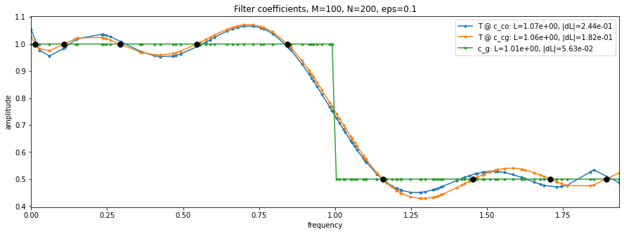
如果对切比雪夫感到陌生,作者还贴心的写了个learning_filter的notebook,这里面讲了有无参数下用梯度下降和sgd等优化的影响,比如说如何用Chebyshev expansion来近似一个滤波器函数 g g g 的方法和结果,可视化结果为:
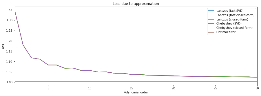
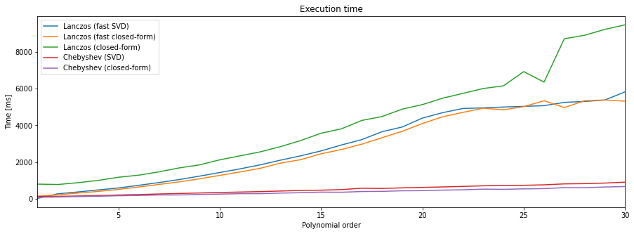
以及关于Lanczos和Chebyshev两种方法的比较,Lanczos和Chebyshev都是用于求解稀疏矩阵特征值问题的迭代算法,它们都利用了多项式函数来近似目标特征值。但Lanczos方法使用了正交多项式,而Chebyshev方法使用了切比雪夫多项式,这里作者写了一个demo做对比,可视化结果为:
绕回正题,认识了模型框架,有了卷积计算公式,这里就可以调参了,这里介绍一组mnist训练参数为:
 	name = 'cgconv_softmax'
    params = common.copy()
    params['dir_name'] += name
    params['regularization'] = 0
    params['dropout']        = 1
    params['filter'] = 'chebyshev5'
    params['learning_rate']  = 0.1
    params['decay_rate']     = 0.999
    params['momentum']       = 0
    params['F']              = [5]  # 卷积核的输出维度
    params['K']              = [15]	# 切比雪夫多项式数
    params['p']              = [1]	# 每层池化的pool_size
    params['M']              = [100, C] # 最后的FC层
    model_perf.test(models.cgcnn(L, **params), name, params,
                    train_data, train_labels, val_data, val_labels, test_data, test_labels)
具体的输出日志为:
NN architecture
  input: M_0 = 976
  layer 1: cgconv1
    representation: M_0 * F_1 / p_1 = 976 * 10 / 1 = 9760
    weights: F_0 * F_1 * K_1 = 1 * 10 * 20 = 200
    biases: F_1 = 10
  layer 2: logits (softmax)
    representation: M_2 = 10
    weights: M_1 * M_2 = 9760 * 10 = 97600
    biases: M_2 = 10
step 600 / 11000 (epoch 1.09 / 20):
  learning_rate = 1.90e-02, loss_average = 1.32e-01
  validation accuracy: 95.84 (4792 / 5000), f1 (weighted): 95.84, loss: 1.48e-01
  time: 583s (wall 34s)
......

step 11000 / 11000 (epoch 20.00 / 20):
  learning_rate = 7.55e-03, loss_average = 2.83e-02
  validation accuracy: 98.12 (4906 / 5000), f1 (weighted): 98.12, loss: 6.28e-02
  time: 10839s (wall 637s)
validation accuracy: peak = 98.18, mean = 98.09
INFO:tensorflow:Restoring parameters from /home/runone/program/competition/cnn_graph/lib/../checkpoints/mnist/cgconv_softmax/model-11000
train accuracy: 99.39 (54662 / 55000), f1 (weighted): 99.39, loss: 2.45e-02
time: 404s (wall 21s)
INFO:tensorflow:Restoring parameters from /home/runone/program/competition/cnn_graph/lib/../checkpoints/mnist/cgconv_softmax/model-11000
test  accuracy: 98.13 (9813 / 10000), f1 (weighted): 98.13, loss: 6.46e-02
time: 71s (wall 4s)
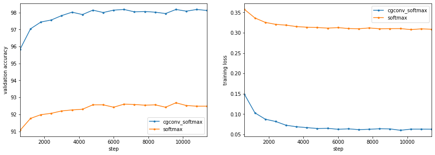
这里单看数据,感觉有些过拟合,但基本差距也不大,可能也是作者随手写得一组数据,因为整个notebook有训练差不多十多组。。。emmm,我就跑了两组,因为我是用CPU跑的,等新闻分类数据集的时候再来说为什么用CPU,最后是可视化,即:
$ model_perf.show()

  accuracy        F1             loss        time [ms]  name
test  train   test  train   test     train
98.13 99.39   98.13 99.39   6.46e-02 2.45e-02    58   cgconv_softmax
92.27 92.30   92.26 92.29   3.13e-01 3.14e-01     3   softmax
到此,是该模型的一个完整流程,看起来没什么坑,只因为我先做的fetch_20newsgroups 数据集,坑就多了,这里简单介绍一些。
首先,包问题,根据现在的tensorflow版本,pypi和其它几个源站都已经不支持tensorflow 2.0以下了,所以需要下载的话,要不用离线包,要不找非主流原地址,这里我大概跑了下,发现即使是tensorflow 1.13都对该项目高了。然后在issues中,发现作者写这个的时候竟然用的tensorflow 1.1.0。。。这是何等的卧槽了,于是开始了痛苦之旅,创建了一个基于python 3.6的新环境,安装requirements,发现它默认安装的tensorflow-gpu,但都2023年了,已经不支持低于8以下的cuda版本,所以只能跑CPU,然后坑就越来越多,emmm
环境没问题后,拉取sklearn的数据,即:
# Fetch dataset. Scikit-learn already performs some cleaning.
remove = ('headers','footers','quotes')  # (), ('headers') or ('headers','footers','quotes')
train = utils.Text20News(data_home=FLAGS.dir_data, subset='train', remove=remove)
这里没有在当前环境安装梯子,sklearn会发送https请求到指定服务器,然后报错为403,解决方案是离线下载数据集,并修改源码进行本地导入,参考:
sklearn.datasets.fetch_20newsgroups的下载速度极慢采用离线下载导入
改完后,需要进行一次embedding,即:
# Word embedding
if True:
    train.embed()
else:
    train.embed(os.path.join('..', 'data', 'word2vec', 'GoogleNews-vectors-negative300.bin'))
train.data_info()
# Further feature selection. (TODO)
这里只能走下面这一句,但是GoogleNews-vectors-negative300.bin 大概有3个多G,在Google drive和kaggle上有资源,其它的我没找到了,我也没下了,就到此为止。整体评价,该作者的notebook写得确实漂亮,不然我也不会有复现的想法,但脱离版本太多,其中还有gensim包的问题,接口已经过时不用了,但看看还是挺好的。
GCN:Graph Convolutional Networks
到这个时期,模型开始模块化,在cs224w的课上,Stanford的导师讲完该节理论后,提出的复现包为pytorch-geometric包,因为是有他参与的,所以主页上就主推了,那本节一样以该包作为对象,但除了参考Stanford,还有唐宇迪的B站视频。
pytorch-geometric包安装
这里需要注意的是该包的安装方式,还是跟上节那样,如果是国内的话,就走离线安装最稳妥,直接安装会有一些bug,具体是啥我忘了,当时没做记录。那么离线安装的步骤如下。
首先,需要安装当前适配版本的torchvision以及torch包,这里最好在最新的前一个版本,因为可能PyG还没有适配好,我这里跟我的服务器的CUDA版本一致,为:
pip3 install torch==1.10.0+cu111 torchvision==0.11.0+cu111
然后去PyG提供的离线包网址找到当前版本的torch:
https://pytorch-geometric.com/whl/
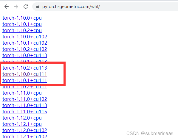
进入确认下之后需要安装的其余几个依赖包的版本,即torch_sparse、torch_cluster、torch_scatter、torch_spline,这里我的安装步骤为:
wget https://data.pyg.org/whl/torch-1.10.0%2Bcu113/torch_cluster-1.6.0-cp38-cp38-linux_x86_64.whl
wget https://data.pyg.org/whl/torch-1.10.0%2Bcu113/torch_scatter-2.0.9-cp38-cp38-linux_x86_64.whl
wget https://data.pyg.org/whl/torch-1.10.0%2Bcu113/torch_sparse-0.6.13-cp38-cp38-linux_x86_64.whl
wget https://data.pyg.org/whl/torch-1.10.0%2Bcu113/torch_spline_conv-1.2.1-cp38-cp38-linux_x86_64.whl

pip install torch_cluster-1.6.0-cp38-cp38-linux_x86_64.whl
pip install torch_scatter-2.0.9-cp38-cp38-linux_x86_64.whl
pip install torch_sparse-0.6.13-cp38-cp38-linux_x86_64.whl
pip install torch_spline_conv-1.2.1-cp38-cp38-linux_x86_64.whl
依赖没有问题后,就能安装pyg的包了:
pip install torch_geometric
安装完成后,这里以跆拳道数据集为例,PyG中直接集成了该数据,版本更新到现在,内部也已经快有100多种额外的各种论文中提到小数据集,这里代码为:
from torch_geometric.datasets import KarateClub

dataset = KarateClub()
print(f'Dataset: {

      dataset}:')
print('======================')
print(f'Number of graphs: {

      len(dataset)}')
print(f'Number of features: {

      dataset.num_features}')
print(f'Number of classes: {

      dataset.num_classes}')

"""
Dataset: KarateClub():
======================
Number of graphs: 1
Number of features: 34
Number of classes: 4
"""
可以取出dataset查看数据结构格式:
data = dataset[0]  # Get the first graph object.
print(data)

"""
Data(x=[34, 34], edge_index=[2, 156], y=[34], train_mask=[34])
"""
其中:
- edge_index:表示图的连接关系(start,end两个序列)
- node features:每个点的特征
- node labels:每个点的标签
- train_mask:有的节点木有标签(用来表示哪些节点要计算损失)
关于其它数据集,也能从torch_geometric.datasets导入,这里就不再进行说明,然后直接看回正题,那么怎么定义一个GCN网络呢?PyG中也有相关文档说明为GCNConv,公式如下:
x v ( ℓ + 1 ) = W ( ℓ + 1 ) ∑ w ∈ N ( v ) ∪ { v } 1 c w , v ⋅ x w ( ℓ ) \mathbf{x}_v^{(\ell + 1)} = \mathbf{W}^{(\ell + 1)} \sum_{w \in \mathcal{N}(v) \, \cup \, \{ v \}} \frac{1}{c_{w,v}} \cdot \mathbf{x}_w^{(\ell)} xv(ℓ+1)=W(ℓ+1)w∈N(v)∪{ v}∑cw,v1⋅xw(ℓ)
代码为:
import torch
from torch.nn import Linear
from torch_geometric.nn import GCNConv


class GCN(torch.nn.Module):
    def __init__(self):
        super().__init__()
        torch.manual_seed(1234)
        self.conv1 = GCNConv(dataset.num_features, 4) # 只需定义好输入特征和输出特征即可
        self.conv2 = GCNConv(4, 4)
        self.conv3 = GCNConv(4, 2)
        self.classifier = Linear(2, dataset.num_classes)

    def forward(self, x, edge_index):
        h = self.conv1(x, edge_index) # 输入特征与邻接矩阵(注意格式,上面那种)
        h = h.tanh()
        h = self.conv2(h, edge_index)
        h = h.tanh()
        h = self.conv3(h, edge_index)
        h = h.tanh()

        # 分类层
        out = self.classifier(h)

        return out, h

model = GCN()
print(model)
这里以上面的跆拳道数据进行训练,首先看看当前一次GCN的可视化图像为:
model = GCN()

_, h = model(data.x, data.edge_index)
print(f'Embedding shape: {

      list(h.shape)}')

visualize_embedding(h, color=data.y)

然后大概训练10次后的样子为:
import time

model = GCN()
criterion = torch.nn.CrossEntropyLoss()  # Define loss criterion.
optimizer = torch.optim.Adam(model.parameters(), lr=0.01)  # Define optimizer.

def train(data):
    optimizer.zero_grad()
    out, h = model(data.x, data.edge_index) #h是两维向量,主要是为了咱们画个图
    loss = criterion(out[data.train_mask], data.y[data.train_mask])  # semi-supervised
    loss.backward()
    optimizer.step()
    return loss, h

for epoch in range(401):
    loss, h = train(data)
    if epoch % 10 == 0:
        visualize_embedding(h, color=data.y, epoch=epoch, loss=loss)
        time.sleep(0.3)
(PS:这里当时跑的时候,容器被删了,emmm,restart了一下把我装的包全还原了,我也就没保存到原图)
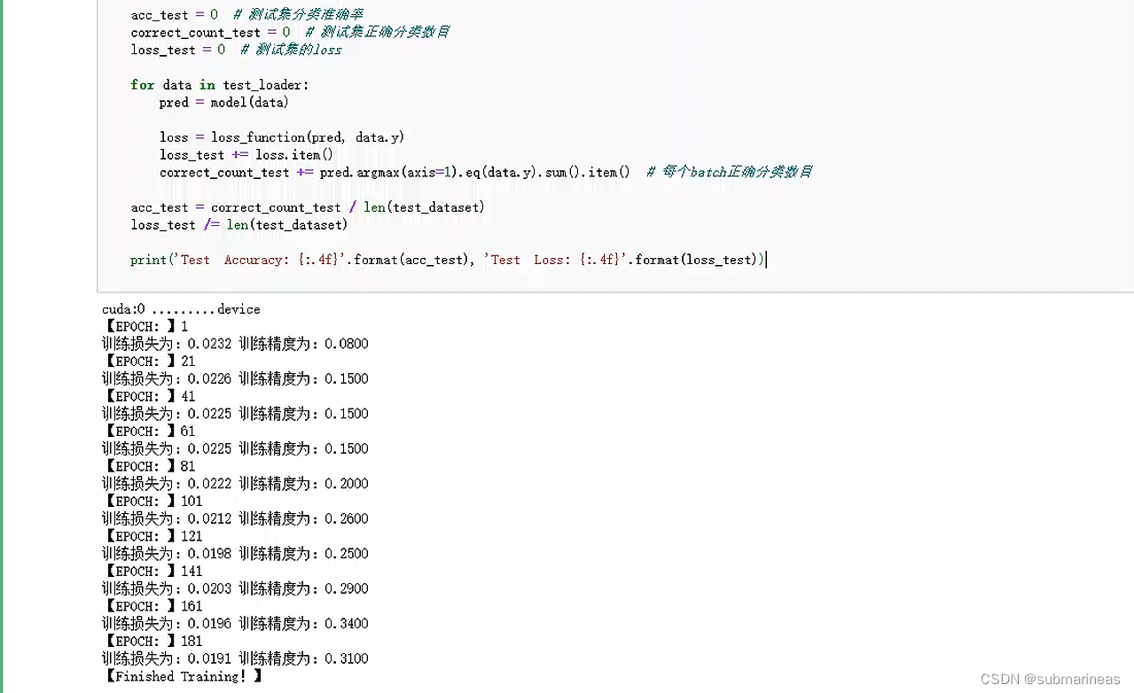
以及跟上面两节一样,使用mnist数据集做GCN网络分类,这里可以参考github上有个mnistGNN的项目,当然还有本站另一个博主的链接:
https://blog.csdn.net/m0_47256162/article/details/128961191
其实GCN也很简单,在pyg中跟pytorch定义一个CNN步骤基本一致,除了GCN类外,其它训练、定义损失等等,就不再赘述,这里我参考上面那篇链接跑了一下,还行:
另外,还有很多其它的实现集成GCN网络的包,比如说pygcn,或者dgl,这些都对GCN 了不同程度的优化,链接如下:
https://github.com/dmlc/dgl
https://github.com/tkipf/pygcn
这里如果之后有遇到相关模型用上述链接包,会回头再这里补充一下,使用经验,那么本篇到此结束。